Appendix
Prerequisites
library("tidyverse")
library("stringr")
library("bayz")
20.14 Parameters
| Category | Description |
|---|---|
| modeled data | Data, assigned distribution |
| unmodeled data | Data not given a distribution |
| modeled parameters | Parameters with an informative prior distribution |
| unmodeled parameters | Parameters with non-informative prior distribution |
| derived quantities | Variables defined deterministicically |
See A. Gelman and Hill (2007, 366)
20.15 Miscellaneous Mathematical Background
20.15.1 Location-Scale Families
In a location-scale family of distributions, if the random variable \(X\) is distributed with mean 0 and standard deviation 1, then the random variable \(Y\), \[ Y = \mu + \sigma X , \] has mean \(\mu\) and standard deviation \(\sigma\).
Normal distribution: Suppose \(X \sim \dnorm(0, 1)\), then \[ Y = \mu + \sigma X, \] is equivalent to \(Y \sim \dnorm(\mu, \sigma)\) (normal with mean \(\mu\) and standard deviation \(\sigma\)).
** Student-t distribution** (including Cauchy): \[ \begin{aligned}[t] X &\sim \dt{\nu}(0, 1) \\ Y &= \mu + \sigma X \end{aligned} \] implies \[ Y \sim \dt{\nu}(\mu, \sigma), \] i.e. \(Y\) is distributed Student-\(t\) with location \(\mu\) and scale \(\sigma\).
In Stan, it can be useful parameterize distributions in terms of a mean 0, scale 1 parameters, and separate parameters for the locations and scales. E.g. with normal distributions,
parameters {
  real mu;
  real<lower = 0.0> sigma;
  vector[n] eps;
}
transformed parameters {
  vector[n] y;
  y = mu + sigma * eps;
}
model {
  eps ~ normal(0.0, 1.0);
}
20.15.2 Scale Mixtures of Normal Distributions
Some commonly used distributions can be represented as scale mixtures of normal distributions. For formal details of scale mixtures of normal distributions see West (1987). Distributions that are scale-mixtures of normal distributions can be written as, \[ Y \sim \dnorm(\mu, \sigma_i^2) \\ \sigma_i \sim \pi(\sigma_i) \] As its name suggests, the individual variances (scales) themselves, have a distribution.
Some examples:
- Student-t
- Double Exponential
- Horseshoe or Hierarchical Shrinkage (HS)
- Horseshoe Plus or Hierarchical Shrinkage Plus (HS+)
Even when analytic forms of the distribution are available, representing them as scale mixtures of normal distributions may be convenient in modeling. In particular, it may allow for drawing samples from the distribution easily. And in HMC, it may induce a more tractable posterior density.
20.15.3 Covariance-Correlation Matrix Decomposition
The suggested method for modeling covariance matrices in Stan is the separation strategy which decomposes a covariance matrix \(\Sigma\) can be decomposed into a standard deviation vector \(\sigma\), and a correlation matrix \(R\) (Barnard, McCulloch, and Meng 2000), \[ \Sigma = \diag(\sigma) R \diag(\sigma) . \] This is useful for setting priors on covariance because separate priors can be set for the scales of the variables via \(\sigma\), and the correlation between them, via \(R\).
The rstanarm decov prior goes further and decomposes the covariance matrix into a correlation matrix, \(\mat{R}\),
a diagonal variance matrix \(\mat{\Omega}\) with trace \(n \sigma^2\), a scalar global variance \(\sigma^2\), and a simplex \(\vec{\pi}\) (proportion of total variance for each variable):
\[
\begin{aligned}[t]
\mat{\Sigma} &= \mat{\Omega} \mat{R} \\
\diag(\mat{\Omega}) &= n \vec{\pi} \sigma^2
\end{aligned}
\]
Separate and interpretable priors can be put on \(\mat{R}\), \(\vec{\pi}\), and \(\sigma^2\).
The LKJ (Lewandowski, ) distribution is a distribution over correlation coefficients, \[ R \sim \dlkjcorr(\eta) , \] where \[ \dlkjcorr(\Sigma | \eta) \propto \det(\Sigma)^{(\eta - 1)} . \]
This distribution has the following properties:
- \(\eta = 1\): uniform correlations
- \(\eta \to \infty\): approaches the identity matrix
- \(0 < \eta < 1\): there is a trough at the identity matrix with higher probabilities placed on non-zero correlations.
- For all positive \(\eta\) (\(\eta > 0\)), \(\E(R) = \mat{I}\).
lkjcorr_df <- function(eta, n = 2) {
  out <- as.data.frame(rlkjcorr(n, eta))
  out$.row <- seq_len(nrow(out))
  out <- gather(out, .col, value, -.row)
  out$.col <- as.integer(str_replace(out$.col, "^V", ""))
  out$eta <- eta
  out
}

lkjsims <- purrr::map_df(c(0.01, 0.1, 1, 2, 50, 1000), lkjcorr_df, n = 50)
This simulates a single matrix from the LKJ distribution with different values of \(\eta\). As \(\eta \to \infty\), the off-diagonal correlations tend towards 0, and the correlation matrix to the identity matrix.
ggplot(lkjsims,
       aes(x = .row, y = .col, fill = value)) +
  facet_wrap(~ eta, ncol = 2) +
  scale_fill_distiller(limits = c(-1, 1), type = "div", palette = "RdYlBu") +
  geom_raster() +
  theme_minimal() +
  theme(panel.grid = element_blank(), axis.text = element_blank()) +
  labs(x = "", y = "")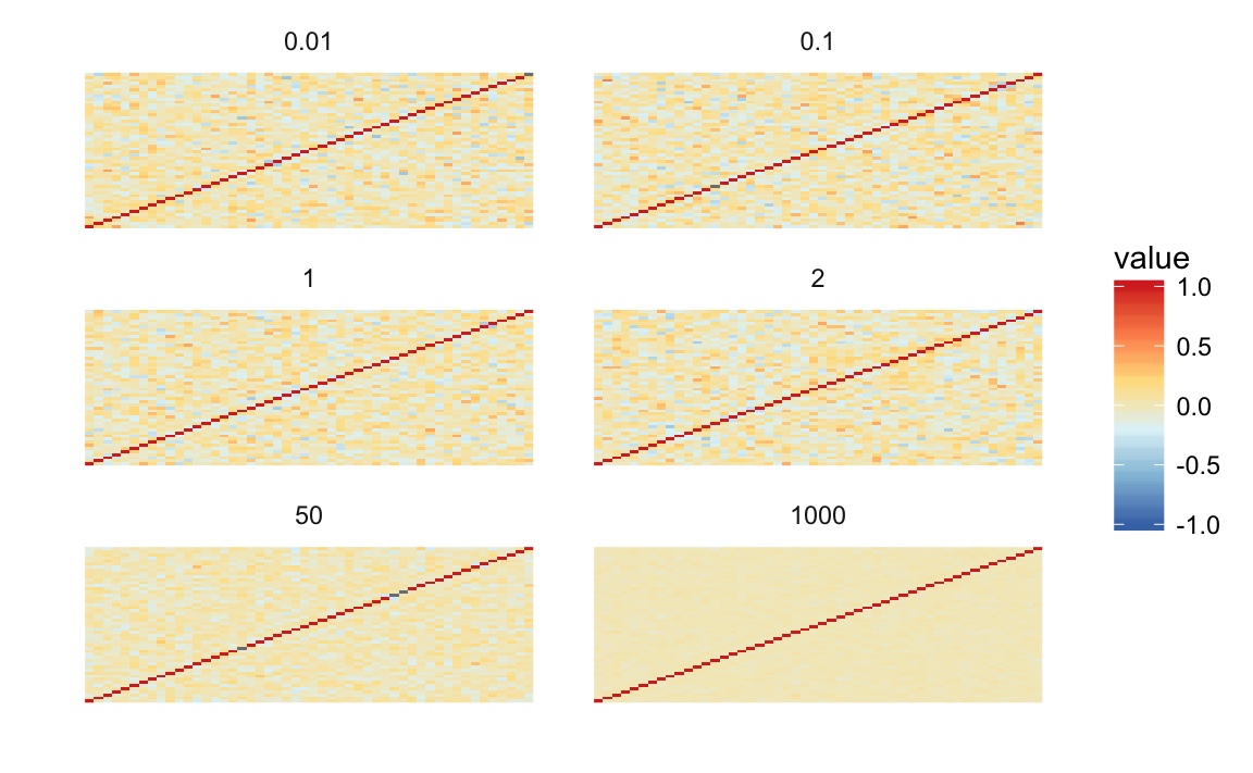
The density of the off-diagonal correlations.
lkjsims %>%
  filter(.row < .col) %>%
  ggplot(aes(x = value, colour = factor(eta))) +
  geom_density()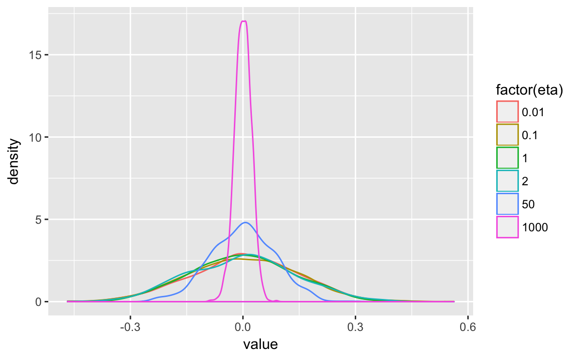
For other discussions of the LKJ correlation distribution, see these:
20.15.4 QR Factorization
For a full-rank \(N \times K\) matrix, the QR factorization is \[ \mat{X} = \mat{Q} \mat{R} \] where \(\mat{Q}\) is an orthonormal matrix such that \(\mat{Q}\T \mat{Q}\) and \(\mat{R}\) is an upper triangular matrix.
Stan function Stan Development Team (2016) suggest writing it is \[ \begin{aligned}[t] \mat{Q}^* = \mat{Q} \times \sqrt{N - 1} \\ \mat{R}^* = \frac{1}{\sqrt{N - 1}} \mat{R} \end{aligned} \]
This is used for solving linear model.
Suppose \(\vec{\beta}\) is a \(K \times 1\) vector, then \[ \vec{eta} = \mat{x} \vec{\beta} = \mat{Q} \mat{R} \vec{\beta} = \mat{Q}^* \mat{R}^* \vec{\beta} . \] Suppose \(\mat{theta} = \mat{R}^* \vec{\beta}\), then \(\vec{eta} = \mat{Q}^* \mat{\theta}\) and \(\vec{beta} = {\mat{R}^*}^{-1} \mat{\theta}\).
rstanarm provides a prior for a normal linear model which uses the QR decomposition to parameterize a prior in terms of \(R^2\).
Stan functions:
qr_Q(matrix A)qr_R(matrix A)
See Stan Development Team (2016 Sec 8.2)
20.15.5 Cholesky Decomposition
The Cholesky decomposition of a positive definite matrix \(A\) is, \[ \mat{A} = \mat{L} \mat{L}\T , \] where \(\mat{L}\) is a lower-triangular matrix.
- It is similar to a square root for a matrix.
It often more numerically stable or efficient to work with the Cholesky decomposition, than with a covariance matrix. When working with the covariance matrix, numerical precision can result in a non positive definite matrix. However, working with \(\mat{L}\) will ensure that \(\mat{A} = \mat{L} \mat{L}\T\) will be positive definite.
In Stan
- Types types
cholesky_factor_cov, andcholesky_factor_corrrepresent the Cholesky factor of covariance and correlation matrices, respectively. - Cholesky decomposition function is
cholesky_decompose(matrix A)
- Types types
Multiple functions in Stan are parameterized with Cholesky decompositions instead of or in addition to covariance matrices. Use them if possible; they are more numerically stable.
lkj_corr_chol_lpdfmulti_normal_cholesky_lpdf
The Cholesky factor is used for sampling from a multivariate normal distribution using i.i.d. standard normal distributions. Suppose \(X_1, \dots, X_N\) are \(N\) i.i.d. standard normal distributions, \(\mat{\Omega}\) is an \(N \times N\) lower-triangular matrix such that \(\mat{\Omega} \mat{Omega}\T = \mat{\Sigma}\), and \(\mu\) is an \(N \times 1\) vector, then \[ \vec{\mu} + \mat{\Omega} X \sim \dnorm(\vec{\mu}, \mat{\Sigma}) \]
See Stan Development Team (2016, 40, 147, 241, 246)
20.16 Scaled and Unscaled Variables
Though priors shouldn’t depend on the data itself, many priors depends
Suppose \(\tilde{Y}\), \(\tilde{X}\), \(\tilde{\alpha}\), \(\tilde{\beta}\), and \(\epsilon\) are random variables, such that \[ \tilde{Y} = \tilde{\alpha} + \tilde{\beta} \tilde{X} + \epsilon . \] These random variables have the following properties, \[ \begin{aligned}[t] \tilde{Y} &= \frac{Y - \bar{Y}}{\sigma_Y}, & \E[\tilde{Y}] &= 0, & \sigma_Y^2 &= \Var[\tilde{Y}] = 1 \\ \tilde{X} &= \frac{X - \bar{X}}{\sigma_X}, & \E[\tilde{X}] &= 0, & \sigma_X^2 &= \Var[\tilde{X}] = 1 , \\ && \E[\epsilon] &= 0 & \sigma_{\tilde{\epsilon}}^2 &= \Var[\tilde{\epsilon}] \end{aligned} \] where \[ \begin{aligned}[t] \bar{X} &= \E[X] , & s_X^2 &= \Var[X] , \\ \bar{Y} &= \E[Y] , & s_Y^2 &= \Var[Y] . \end{aligned} \]
Then via some algebra, \[ \begin{aligned} Y &= \underbrace{\sigma_{Y} \tilde{\alpha} + \bar{Y} - \frac{\sigma_Y }{\sigma_X} \tilde{\beta} \bar{X}}_{\alpha} + \underbrace{\frac{\sigma_Y}{\sigma_X} \tilde{\beta}}_{\beta} X + \underbrace{\sigma_Y \tilde{\epsilon}}_{\epsilon} \\ &= \alpha + \beta X + \epsilon . \end{aligned} \] The primary relationships of interest are those between \(\alpha\) and \(\tilde{\alpha}\), \(\beta\) and \(\tilde{\beta}\), and \(\epsilon\) and \(\tilde{\epsilon}\). These can be used to convert between coefficients estimated with standardized data to the coefficients on the data scale, or to adjust scale-free weakly informative priors to the data scale. \[ \begin{aligned}[t] \tilde{\alpha} &= \sigma_Y^{-1}\left(\alpha - \bar{Y} + \beta \bar{X} \right) \\ &= \sigma_Y^{-1}\left(\alpha - \bar{Y} + \frac{\sigma_Y}{\sigma_X} \tilde{\beta} \bar{X} \right), \\ \alpha &= \sigma_Y \tilde{\alpha} + \bar{Y} - \frac{\sigma_Y}{\sigma_X} \tilde{\beta} \bar{X} \\ &= \sigma_Y \tilde{\alpha} + \bar{Y} - \beta \bar{X} , \\ \tilde{\beta} &= \frac{\sigma_X}{\sigma_Y} \beta , \\ \beta &= \frac{\sigma_Y}{\sigma_X} \tilde{\beta} , \\ \tilde{\epsilon} &= \epsilon / \sigma_Y , \\ \epsilon &= \sigma_Y \tilde{\epsilon} . \end{aligned} \] This implies the following relationships between their means and variances, \[ \begin{aligned}[t] E(\alpha) &= \sigma_{Y} E(\tilde{\alpha}) + \bar{Y} - \frac{\sigma_Y}{\sigma_X} E(\tilde{\beta}) \bar{X} , & V(\alpha) &= \sigma_{Y}^2 V(\tilde{\alpha}) + \frac{\sigma_Y^2}{\sigma_X^2} V(\tilde{\beta}) \bar{X}^2 , \\ &= \sigma_{Y} E(\tilde{\alpha}) + \bar{Y} - \bar{X} E(\beta) , & &= \sigma_{Y}^2 V(\tilde{\alpha}) + \bar{X}^2 V(\beta) , \\ E(\tilde{\alpha}) &= \frac{E(\alpha) - \bar{Y} + E(\beta) \bar{X} }{\sigma_Y} , & V(\tilde{\alpha}) &= \sigma_Y^{-2} \left[ V(\alpha) + \bar{X}^2 V(\beta) \right] \end{aligned} \] For example, a weakly informative prior on \(\tilde{\alpha}\) implies a prior on \(\alpha\), \[ \tilde{\alpha} \sim N(0, 10^2) \to \alpha \sim N \left( \frac{\beta \bar{X} - \bar{Y}}{\sigma_Y}, \sigma_Y^2 10^2 \right) . \]
\[ \begin{aligned}[t] E(\beta) &= \frac{\sigma_Y}{\sigma_X} E(\tilde{\beta}) , & V(\beta) &= \frac{\sigma_Y^2}{\sigma_X^2} V(\tilde{\beta}) , \\ E(\tilde{\beta}) &= \frac{\sigma_X}{\sigma_Y} E(\beta) , & V(\tilde{\beta}) &= \frac{\sigma_X^2}{\sigma_Y^2} V(\beta) . \end{aligned} \]
For example, a weakly informative prior on \(\tilde{\beta}\) implies the following prior on \(\beta\), \[ \tilde{\beta} \sim N(0, 2.5^2) \to \beta \sim N\left(0, \frac{\sigma_Y^2}{\sigma_X^2} 2.5^2 \right) . \]
\[ \begin{aligned}[t] E(\epsilon) &= 0 , & V(\epsilon) &= \sigma_Y^2 V(\tilde{\epsilon}), \\ E(\tilde{\epsilon}) &= 0 , & V(\tilde{\epsilon}) &= \sigma_Y^{-2} V(\epsilon) . \end{aligned} \] For example, a weakly informative prior on the variance of \(\tilde{\epsilon}\) implies a weakly informative prior on the variance of \(\epsilon\), \[ \sigma_{\tilde{\epsilon}} \sim C^{+}\left(0, 5 \right) \to \sigma_{\epsilon} \sim C^{+}\left(0, 5 \sigma_Y \right) . \]