\[ \DeclareMathOperator{\E}{E} \DeclareMathOperator{\mean}{mean} \DeclareMathOperator{\Var}{Var} \DeclareMathOperator{\Cov}{Cov} \DeclareMathOperator{\Cor}{Cor} \DeclareMathOperator{\Bias}{Bias} \DeclareMathOperator{\MSE}{MSE} \DeclareMathOperator{\RMSE}{RMSE} \DeclareMathOperator{\sd}{sd} \DeclareMathOperator{\se}{se} \DeclareMathOperator{\tr}{tr} \DeclareMathOperator{\median}{median} \DeclareMathOperator{\rank}{rank} \DeclareMathOperator*{\argmin}{arg\,min} \DeclareMathOperator*{\argmax}{arg\,max} \DeclareMathOperator{\logistic}{Logistic} \DeclareMathOperator{\logit}{Logit} \newcommand{\mat}[1]{\boldsymbol{#1}} \newcommand{\vec}[1]{\boldsymbol{#1}} \newcommand{\T}{'} % This follows BDA \newcommand{\dunif}{\mathsf{Uniform}} \newcommand{\dnorm}{\mathsf{Normal}} \newcommand{\dhalfnorm}{\mathrm{HalfNormal}} \newcommand{\dlnorm}{\mathsf{LogNormal}} \newcommand{\dmvnorm}{\mathsf{Normal}} \newcommand{\dgamma}{\mathsf{Gamma}} \newcommand{\dinvgamma}{\mathsf{InvGamma}} \newcommand{\dchisq}{\mathsf{ChiSquared}} \newcommand{\dinvchisq}{\mathsf{InvChiSquared}} \newcommand{\dexp}{\mathsf{Exponential}} \newcommand{\dlaplace}{\mathsf{Laplace}} \newcommand{\dweibull}{\mathsf{Weibull}} \newcommand{\dwishart}{\mathsf{Wishart}} \newcommand{\dinvwishart}{\mathsf{InvWishart}} \newcommand{\dlkj}{\mathsf{LkjCorr}} \newcommand{\dt}{\mathsf{StudentT}} \newcommand{\dhalft}{\mathsf{HalfStudentT}} \newcommand{\dbeta}{\mathsf{Beta}} \newcommand{\ddirichlet}{\mathsf{Dirichlet}} \newcommand{\dlogistic}{\mathsf{Logistic}} \newcommand{\dllogistic}{\mathsf{LogLogistic}} \newcommand{\dpois}{\mathsf{Poisson}} \newcommand{\dBinom}{\mathsf{Binomial}} \newcommand{\dmultinom}{\mathsf{Multinom}} \newcommand{\dnbinom}{\mathsf{NegativeBinomial}} \newcommand{\dnbinomalt}{\mathsf{NegativeBinomial2}} \newcommand{\dbetabinom}{\mathsf{BetaBinomial}} \newcommand{\dcauchy}{\mathsf{Cauchy}} \newcommand{\dhalfcauchy}{\mathsf{HalfCauchy}} \newcommand{\dbernoulli}{\mathsf{Bernoulli}} \newcommand{\R}{\mathbb{R}} \newcommand{\Reals}{\R} \newcommand{\RealPos}{\R^{+}} \newcommand{\N}{\mathbb{N}} \newcommand{\Nats}{\N} \newcommand{\cia}{\perp\!\!\!\perp} \DeclareMathOperator*{\plim}{plim} \DeclareMathOperator{\invlogit}{Inv-Logit} \DeclareMathOperator{\logit}{Logit} \DeclareMathOperator{\diag}{diag} \]

13 Binomial Models

Prerequisites

library("rstan")
library("rstanarm")
library("tidyverse")
library("recipes")
library("bayz")

13.1 Introduction

Binomial models are used to an outcome that is a bounded integer, \[ y_i \in 0, 1, 2, \dots, n . \] The outcome is distributed Binomial, \[ \begin{aligned}[t] y_i \sim \dBinom \left(n_i, \pi \right) \end{aligned} \]

A binary outcome is a common special case, \[ y_i \in \{0, 1\}, \] and \[ \begin{aligned}[t] y_i &\sim \dBinom \left(1, \pi \right) & \text{for all $i$} \\ \end{aligned} \]

Depending on the link function, these are logit and probit models that appear in the literature.

13.2 Link Functions {link-function}

The parameter \(\pi \in (0, 1)\) is often modeled with a link function is and a linear predictor. \[ \pi_i = g^{-1}(\vec{x}_i \vec{\beta}) \]

There are several common link functions, but they all have to map \(R \to (0, 1)\).⁷

• Logit: The logistic function, \[ \pi_i = \logistic(x_i\T \beta) = \frac{1}{1 + \exp(- x_i\T\beta)} . \] Stan function softmax.

• Probit: The CDF of the normal distribution. \[ \pi_i = \Phi(x_i\T \beta) \] Stan function normal_cdf.

• cauchit: The CDF of the Cauchy distribution. Stan function cauchy_cdf.

• cloglog: The inverse of the conditional log-log function (cloglog) is \[ \pi_i = 1 - \exp(-\exp(x_i\T \beta)) . \] Stan function inv_cloglog.

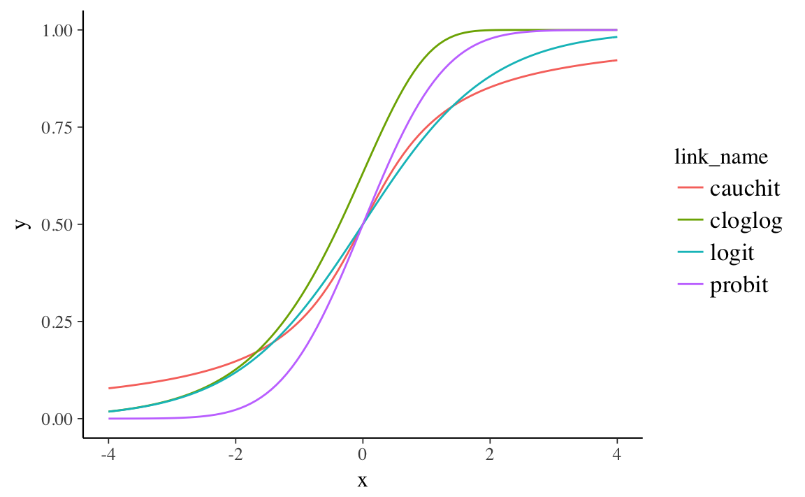
Of these link functions, the probit has the narrowest tails (sensitivity to outliers), followed by the logit, and cauchit. The cloglog function is different in that it is asymmetric.⁸ At zero its value is above 0.5, whereas the cauchit, logit, and probit links all equal 0.5 at 0,

make.link("cloglog")$linkinv(0)
#> [1] 0.632

map(c("logit", "probit", "cauchit", "cloglog"),  make.link) %>%
map_df(
  function(link) {
    tibble(x = seq(-4, 4, length.out = 101),
           y = link$linkinv(x),
           link_name = link$name)
  }
  ) %>%
  ggplot(aes(x = x, y = y, colour = link_name)) +
  geom_line()

Notes:

• The logistic distribution is approximately a Student-t with df=7.

13.2.1 Stan

In Stan, the Binomial distribution has two implementations:

• binomial_lpdf
• binomial_logit_lpdf.

The later implementation is for numeric stability. Taking an exponential of a value can be numerically unstable, and binomial_logit_lpdf input is on the logit scale: Whereas, \[ y_i \sim \mathsf{binomial}(1 / (1 + \exp(x_i \beta))) \] the following is true, \[ y_i \sim \mathsf{binomial\_logit}(x_i \beta) \]

13.2.2 Example: Vote Turnout

Estimate a model of vote turnout in the 1992 from the American National Election Survey (ANES) as a function of race, age, and education. The data and example is from the Zelig library Zelig.⁹ You can load it with

data("turnout", package = "ZeligData")

13.2.3 Stan

A general Stan model for estimating logit models is:

// bernoulli_logit_1.stan
data {
  // number of observations
  int N;
  // response
  // vectors are only real numbers
  // need to use an array
  int y[N];
  // number of columns in the design matrix X
  int K;
  // design matrix X
  // should not include an intercept
  matrix [N, K] X;
  // priors on regression coefficients
  real scale_alpha;
  vector[K] scale_beta;
  // keep responses
  int use_y_rep;
  int use_log_lik;
}
parameters {
  // regression coefficient vector
  real alpha;
  vector[K] beta;
}
transformed parameters {
  vector[N] eta;

  eta = alpha + X * beta;
}
model {
  // priors
  alpha ~ normal(0., scale_alpha);
  beta ~ normal(0., scale_beta);
  // likelihood
  y ~ bernoulli_logit(eta);
}
generated quantities {
  // simulate data from the posterior
  vector[N * use_y_rep] y_rep;
  // log-likelihood posterior
  vector[N * use_log_lik] log_lik;
  for (i in 1:num_elements(y_rep)) {
    y_rep[i] = bernoulli_rng(inv_logit(eta[i]));
  }
  for (i in 1:num_elements(log_lik)) {
    log_lik[i] = bernoulli_logit_lpmf(y[i] | eta[i]);
  }
}

data("turnout", package = "ZeligData")

Vote choice (vote) is modeled as a function of age, age-squared, income, and race.

Preprocess the data to create the design matrix, X, and the response y using the recipes package. We will need to center and scale the design matrix.

turnout <- mutate(turnout, white = as.numeric(race == "white"))
rec_turnout <- recipe(vote ~ income + age + white,
                      data = turnout) %>%
  step_poly(age, options = list(degree = 2)) %>%
  prep(data = turnout, retain = TRUE)
X <- juice(rec_turnout, all_predictors(), composition = "matrix")
y <- juice(rec_turnout, all_outcomes(), composition = "matrix") %>%
  drop()

mod1_data <- list(
  X = X,
  N = nrow(X),
  K = ncol(X),
  y = y,
  scale_alpha = 10,
  scale_beta = 2.5 * apply(X, 2, sd),
  use_y_rep = FALSE,
  use_log_lik = TRUE
)

13.2.3.1 rstanarm

The rstanarm package can estimate binomial models using the function stan_glm:

fit2 <- stan_glm(vote ~ income + age + white, data = turnout)

13.3 References

For general references on binomial models see Stan Development Team (2016 Sec. 8.5), McElreath (2016 Ch 10), A. Gelman and Hill (2007) [Ch. 5; Sec 6.4-6.5], Fox (2016 Ch. 14), and A. Gelman, Carlin, et al. (2013 Ch. 16).

---

7. Since the cumulative distribution function of a distribution maps reals to \((0, 1)\), any CDF can be used as a link function.↩

8. Beck, Katz, and Tucker (1998) show that the cloglog link function can be derived from a grouped duration model with binary response variables.↩

9. Example from Zelig-logit.↩