9 Legislators: Estimating Legislators’ Ideal Points From Voting Histories
library("pscl")
library("tidyverse")
library("forcats")
library("stringr")
library("rstan")
library("sn")
Recorded votes in legislative settings (roll calls) are often used to recover the underlying preferences of legislators.7 Political scientists analyze roll call data using the Euclidean spatial voting model: each legislator (\(i = 1, ..., n\)) has a preferred policy position (\(x_i\), a point in low-dimensional Euclidean space), and each vote (\(j = 1, ..., m\)) amounts to a choice between “Aye” and a “Nay” locations, \(q_j\) and \(Y_j\), respectively. Legislators are assumed to choose on the basis of utility maximization, with utilities (in one-dimension)
In these models, the only observed data are votes, and the analyst wants to model those votes as a function of legislator- (\(\xi_i\)), and vote-specific (\(\alpha_i\), \(\beta_i\)) parameters. The vote of legislator \(i\) on roll-call \(j\) (\(y_{i,j}\)) is a function of a the legislator’s ideal point (\(\xi_i\)), the vote’s cutpoint (\(\alpha_j\)), and the vote’s discrimination (\(\beta_j\)): \[ \begin{aligned}[t] y_{i,j} &\sim \mathsf{Bernoulli}(\pi_i) \\ \pi_i &= \frac{1}{1 + \exp(-\mu_{i,j})} \\ \mu_{i,j} &= \beta_j \xi_i - \alpha_j \end{aligned} \]
9.1 Identification
Ideal points (like many latent space models) are unidentified. In particular, there are three types of invariance:
- Additive aliasing
- Multiplicative aliasing
- Rotation (reflection) invariance
Scale invariance: \[ \begin{aligned}[t] \mu_{i,j} &= \alpha_j + \beta_j \xi_i \\ &= \alpha_j + \left(\frac{\beta_j}{c}\right) \left(\xi_i c \right) \\ &= \alpha_j + \beta^*_j \xi^*_i \end{aligned} \]
Addition invariance: \[ \begin{aligned}[t] \mu_{i,j} &= \alpha_j + \beta_j \xi_i \\ &= \alpha_j - \beta_j c + \beta_j c + \beta_j \xi_i \\ &= (\alpha_j - \beta_j c) + \beta_j (\xi_i + c) \\ &= \alpha_j^{*} + \beta_j \xi^{*}_i \end{aligned} \]
Rotation invariance: \[ \begin{aligned}[t] \mu_{i,j} &= \alpha_j + \beta_j \xi_i \\ &= \alpha_j + \beta_j (-1) (-1) \xi_i \\ &= \alpha_j + (-\beta_j) (-\xi_i) \\ &= \alpha_j + \beta_j^{*} \xi^{*}_i \end{aligned} \]
Example:
xi <- c(-1, -0.5, 0.5, 1)
alpha <- c(1, 0, -1)
beta <- c(-0.5, 0, 0.5)
y <- matrix(c(1, 0, 1, 0, 0, 1, 1, 1, 1, 0, 1, 1), 3, 4)
k <- 1

list(sum(plogis(y - (alpha + beta %o% xi))),
     sum(plogis(y - (alpha + -beta %o% -xi))),
     sum(plogis(y - ((alpha - beta * k) + beta %o% (xi + k)))),
     sum(plogis(y - ((alpha + (beta / k) %o% (xi * k))))))
#> [[1]]
#> [1] 7.5
#>
#> [[2]]
#> [1] 7.5
#>
#> [[3]]
#> [1] 7.5
#>
#> [[4]]
#> [1] 7.5
For each of these: Which types of rotation does it solve?
- Fix one element of \(\beta\).
- Fix one element of \(\xi\).
- Fix one element of \(\alpha\).
- Fix two elements of \(\alpha\).
- Fix two elements of \(\xi\).
- Fix two elements of \(\beta\).
9.2 109th Senate
This example models the voting of the 109th U.S. Senate. Votes for the 109th Senate is included in the pscl package:
The s109 object is not a data frame, so see its documentation for information about its structure.
s109
#> Description:  109th U.S. Senate
#> Source:       ftp://voteview.com/dtaord/sen109kh.ord
#> Number of Legislators:    102
#> Number of Votes:  645
#>
#> Using the following codes to represent roll call votes:
#> Yea:      1 2 3
#> Nay:      4 5 6
#> Abstentions:  7 8 9
#> Not In Legislature:   0
#>
#> Legislator-specific variables:
#> [1] "state"      "icpsrState" "cd"         "icpsrLegis" "party"
#> [6] "partyCode"
#> Vote-specific variables:
#> [1] "date"        "session"     "number"      "bill"        "question"
#> [6] "result"      "description" "yeatotal"    "naytotal"
#> Detailed information is available via the summary function.
This data includes all roll-call votes, votes in which the responses of the senators are recorded.
For simplicity, the ideal point model uses binary responses, but the s109
data includes multiple codes for response
to roll-calls.
1 | Yea |
2 | Paired Yea |
3 | Announced Yea |
4 | Announced Nay |
5 | Paired Nay |
6 | Nay |
7 | Present (some Congresses, also not used some Congresses) |
8 | Present (some Congresses, also not used some Congresses) |
6 | Nay |
9 | Not Voting |
In the data processing, we will aggregate the responses into “Yes”, “No”, and missing values.
close: Definition of non-lopsided votes in ; votes with between 35% and 65% yeas in which the parties are likely to whip members.lopsided: Definition of lopsided votes used in W-NOMINATE and dropped. Votes with less than 2.5% or greater than 97.5% yeas.
s109_vote_data <- as.data.frame(s109$vote.data) %>%
  mutate(rollcall = paste(session, number, sep = "-"),
         passed = result %in% c("Confirmed", "Agreed To", "Passed"),
         votestotal = yeatotal + naytotal,
         yea_pct = yeatotal / (yeatotal + naytotal),
         unanimous = yea_pct %in% c(0, 1),
         close = yea_pct < 0.35 | yea_pct > 0.65,
         lopsided = yea_pct < 0.025 | yea_pct > 0.975) %>%
  filter(!unanimous) %>%
  select(-unanimous) %>%
  mutate(.rollcall_id = row_number())

s109_legis_data <- as.data.frame(s109$legis.data) %>%
  rownames_to_column("legislator") %>%
  mutate(.legis_id = row_number(),
         party = fct_recode(party,
                            "Democratic" = "D",
                            "Republican" = "R",
                            "Independent" = "Indep"))

s109_votes <- s109$votes %>%
  as.data.frame() %>%
  rownames_to_column("legislator") %>%
  gather(rollcall, vote, -legislator) %>%
  # recode to Yea (TRUE), Nay (FALSE), or missing
  mutate(yea = NA,
         yea = if_else(vote %in% c(1, 2, 3), TRUE, yea),
         yea = if_else(vote %in% c(4, 5, 6), FALSE, yea)
         ) %>%
  filter(!is.na(yea)) %>%
  inner_join(dplyr::select(s109_vote_data, rollcall, .rollcall_id), by = "rollcall") %>%
  inner_join(dplyr::select(s109_legis_data, legislator, party, .legis_id), by = "legislator")

partyline <-
  s109_votes %>%
  group_by(.rollcall_id, party) %>%
  summarise(yea = mean(yea)) %>%
  spread(party, yea) %>%
  ungroup() %>%
  mutate(partyline = NA_character_,
         partyline = if_else(Republican < 0.1 & Democratic > 0.9,
                             "Democratic", partyline),
         partyline = if_else(Republican > 0.9 & Democratic < 0.1,
                             "Republican", partyline)) %>%
  rename(pct_yea_D = Democratic, pct_yea_R = Republican) %>%
  select(-Independent)

s109_vote_data <-
  left_join(s109_vote_data, partyline, by = ".rollcall_id")
9.3 Identification by Fixing Legislator’s Ideal Points
Identification of latent state models can be challenging. The first method for identifying ideal point models is to fix the values of two legislators. These can be arbitrary, but if they are chosen along the ideological dimension of interest it can help the substantive interpretation.
Since we know, or expect, that the primary ideological dimension is Liberal-Conservative (Poole and Rosenthal 2000), I’ll fix the ideal points of the two party leaders in that congress. In the 109th Congress, the Republican party was the majority party and Bill Frist (Tennessee) was the majority (Republican) leader, and Harry Reid (Nevada) wad the minority (Democratic) leader: \[ \begin{aligned}[t] \xi_\text{FRIST (R TN)} & = 1 \\ \xi_\text{REID (D NV)} & = -1 \end{aligned} \]
For all of those give a weakly informative prior to the ideal points, and item difficulty and discrimination parameters, \[ \begin{aligned}[t] \xi_{i} &\sim \mathsf{Normal}(\zeta, \tau) \\ \zeta &\sim \mathsf{Normal}(0., 10) \\ \tau &\sim \mathsf{HalfCauchy}(0., 5) \\ \alpha_{j} &\sim \mathsf{Normal}(0, 10) \\ \beta_{j} &\sim \mathsf{Normal}(0, 2.5) && j \in 1, \dots, J \end{aligned} \]
  // ideal point model
// identification:
// - xi ~ hierarchical
// - except fixed senators
data {
  // number of individuals
  int N;
  // number of items
  int K;
  // observed votes
  int Y_obs;
  int y_idx_leg[Y_obs];
  int y_idx_vote[Y_obs];
  int y[Y_obs];
  // priors
  // on items
  real alpha_loc;
  real alpha_scale;
  real beta_loc;
  real beta_scale;
  // on legislators
  int N_xi_obs;
  int idx_xi_obs[N_xi_obs];
  vector[N_xi_obs] xi_obs;
  int N_xi_param;
  int idx_xi_param[N_xi_param];
  // prior on ideal points
  real zeta_loc;
  real zeta_scale;
  real tau_scale;
}
parameters {
  // item difficulties
  vector[K] alpha;
  // item discrimination
  vector[K] beta;
  // unknown ideal points
  vector[N_xi_param] xi_param;
  // hyperpriors
  real tau;
  real zeta;
}
transformed parameters {
  // create xi from observed and parameter ideal points
  vector[Y_obs] mu;
  vector[N] xi;
  xi[idx_xi_param] = xi_param;
  xi[idx_xi_obs] = xi_obs;
  for (i in 1:Y_obs) {
    mu[i] = alpha[y_idx_vote[i]] + beta[y_idx_vote[i]] * xi[y_idx_leg[i]];
  }
}
model {
  alpha ~ normal(alpha_loc, alpha_scale);
  beta ~ normal(beta_loc, beta_scale);
  xi_param ~ normal(zeta, tau);
  xi_obs ~ normal(zeta, tau);
  zeta ~ normal(zeta_loc, zeta_scale);
  tau ~ cauchy(0., tau_scale);
  y ~ bernoulli_logit(mu);
}
generated quantities {
  vector[Y_obs] log_lik;
  for (i in 1:Y_obs) {
    log_lik[i] = bernoulli_logit_lpmf(y[i] | mu[i]);
  }
}
Create a data frame with the fixed values for identification.
Additionally, set initial values of ideal points: Republicans at xi = 1, Democrats at xi = -1, and independents at xi = 0.
This may help speed up convergence.
xi_1 <-
  s109_legis_data %>%
  mutate(
         xi = if_else(legislator == "FRIST (R TN)", 1,
                 if_else(legislator == "REID (D NV)", -1, NA_real_)),
         init = if_else(party == "Republican", 1,
                        if_else(party == "Democratic", -1, 0)))
Define and setup all the data needed for this
legislators_data_1 <-
  within(list(), {
    y <- as.integer(s109_votes$yea)
    y_idx_leg <- as.integer(s109_votes$.legis_id)
    y_idx_vote <- as.integer(s109_votes$.rollcall_id)
    Y_obs <- length(y)
    N <- max(s109_votes$.legis_id)
    K <- max(s109_votes$.rollcall_id)
    # priors
    alpha_loc <- 0
    alpha_scale <- 5
    beta_loc <- 0
    beta_scale <- 2.5
    N_xi_obs <- sum(!is.na(xi_1$xi))
    idx_xi_obs <- which(!is.na(xi_1$xi))
    xi_obs <- xi_1$xi[!is.na(xi_1$xi)]
    N_xi_param <- sum(is.na(xi_1$xi))
    idx_xi_param <- which(is.na(xi_1$xi))
    tau_scale <- 5
    zeta_loc <- 0
    zeta_scale <- 10
})legislators_fit_1 <-
sampling(mod_ideal_point_1, data = legislators_data_1,
chains = 1, iter = 500,
init = legislators_init_1,
refresh = 100,
pars = c("alpha", "beta", "xi"))Extract the ideal point data:
legislator_summary_1 <-
  bind_cols(s109_legis_data,
           as_tibble(summary(legislators_fit_1, par = "xi")$summary)) %>%
mutate(legislator = fct_reorder(legislator, mean))ggplot(legislator_summary_1,
aes(x = legislator, y = mean,
ymin = `2.5%`, ymax = `97.5%`, colour = party)) +
geom_pointrange() +
coord_flip() +
scale_color_manual(values = c(Democratic = "blue", Independent = "gray", Republican = "red")) +
labs(y = expression(xi[i]), x = "", colour = "Party") +
theme(legend.position = "bottom")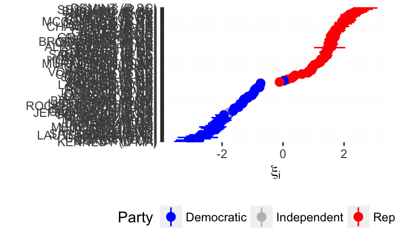
(#fig:legislator_plot_1)Estimated Ideal Points of the Senators of the 109th Congress
9.4 Identification by Fixing Legislator’s Signs
We can identify the scale and location of the latent dimensions by fixing the mean and location of the distribution of the legislator’s ideal points. This can be done by \[ \xi_i \sim \mathsf{Normal}(0, 1) \] This does not exactly fix the mean of \(\xi\) in any particular simulation. As the sample size increases, \(n \to \infty\) will give \(mean(\xi) \to 0\) and \(sd(\xi) \to 1\). This “soft-identification” will also overestimate the uncertainty in the ideal points of legislators (see paper by … ? ). So in the estimation, I do the following to ensure that in each simulation, \(\xi\) has exactly mean 0 and standard deviation 1. \[ \begin{aligned}[t] \xi_i^{*} &\sim \mathsf{Normal}(0, 1) \\ \xi_i &= \frac{\xi^*_i - \mathrm{mean}(\xi)}{\mathrm{sd}(\xi)} \end{aligned} \] However, this does not identify the direction of the latent variables. This can be done by restriction the sign of either a single legislator (\(\xi_i\)) or roll-call (\(\beta_i\)).
In this case, instead of fixing the ideal points of two legislators, instead use skew-normal distributions to set the sides of each legislator. \[ \beta_j \sim \mathsf{SkewNormal}(0, 2.5, d_j ) \] where \[ d_j = \begin{cases} -50 & \text{if Democratic party line vote} \\ 0 & \text{not a party line vote} \\ 50 & \text{if Republican party line vote} \end{cases} . \]
The skew-normal distribution is an extension of the normal distribution with an additional skewness parameter, \[ y \sim \mathsf{SkewNormal}(\mu, \sigma, \alpha) \] as \(|\alpha| \to \infty\), the skew-normal approaches a half-normal distribution.
map_df(c(-50, 0, 50),
        function(alpha) {
          tibble(x = seq(-4, 4, by = 0.1),
                 density = dsn(x, alpha = alpha),
                 alpha = alpha)
        }) %>%
  ggplot(aes(x = x, y = density, colour = factor(alpha))) +
  geom_line()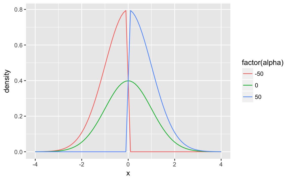
  // ideal point model
// identification:
// - ideal points ~ normal(0, 1)
// - signs of ideal points using skew normal
data {
  // number of individuals
  int N;
  // number of items
  int K;
  // observed votes
  int Y_obs;
  int y_idx_leg[Y_obs];
  int y_idx_vote[Y_obs];
  int y[Y_obs];
  // priors
  // on items
  real alpha_loc;
  real alpha_scale;
  real beta_loc;
  real beta_scale;
  // on ideal points
  vector[N] xi_skew;
}
parameters {
  // item difficulties
  vector[K] alpha;
  // item discrimination
  vector[K] beta;
  // unknown ideal points
  vector[N] xi_raw;
}
transformed parameters {
  // create xi from observed and parameter ideal points
  vector[Y_obs] mu;
  vector[N] xi;

  xi = (xi_raw - mean(xi_raw)) ./ sd(xi_raw);
  for (i in 1:Y_obs) {
    mu[i] = alpha[y_idx_vote[i]] + beta[y_idx_vote[i]] * xi[y_idx_leg[i]];
  }
}
model {
  alpha ~ normal(alpha_loc, alpha_scale);
  beta ~ normal(beta_loc, beta_scale);
  // soft center ideal points
  // in transformed block enforce hard-centering
  xi_raw ~ skew_normal(0., 1., xi_skew);
  y ~ bernoulli_logit(mu);
}
generated quantities {
  vector[Y_obs] log_lik;

  for (i in 1:Y_obs) {
    log_lik[i] = bernoulli_logit_lpmf(y[i] | mu[i]);
  }
}
Instead of fixing the ideal points, set the skewness parameter of the skew normal distribution so that \(\xi_{\text{FRIST (R TN)}} > 0\).
legislators_data_2 <-
  within(list(), {
    y <- as.integer(s109_votes$yea)
    y_idx_leg <- as.integer(s109_votes$.legis_id)
    y_idx_vote <- as.integer(s109_votes$.rollcall_id)
    Y_obs <- length(y)
    N <- max(s109_votes$.legis_id)
    K <- max(s109_votes$.rollcall_id)
    # priors
    alpha_loc <- 0
    alpha_scale <- 5
    beta_loc <- 0
    beta_scale <- 2.5
    xi_skew <- if_else(s109_legis_data$legislator == "FRIST (R TN)", 50, 0)
})9.5 Identification by Discrimination Parameters’ Signs
Alternatively, we can identify the location and scale of the latent dimensions with the legislator’s ideal points, \[ \begin{aligned}[t] \xi_i^{*} &\sim \mathsf{Normal}(0, 1) \\ \xi_i &= \frac{\xi^{*}_i - \mathrm{mean}(\xi)}{\mathrm{sd}(\xi)} , \end{aligned} \] and identify the rotation of latent dimensions by fixing the sign of the discrimination parameter of a single roll-call vote (\(\beta_j\)).
  // ideal point model
//
// identification:
// - ideal points ~ normal(0, 1)
// - signs of item discrimination using skew normal
data {
  // number of individuals
  int N;
  // number of items
  int K;
  // observed votes
  int Y_obs;
  int y_idx_leg[Y_obs];
  int y_idx_vote[Y_obs];
  int y[Y_obs];
  // priors
  // on items
  real alpha_loc;
  real alpha_scale;
  vector[K] beta_loc;
  vector[K] beta_scale;
  vector[K] beta_skew;
}
parameters {
  // item difficulties
  vector[K] alpha;
  // item discrimination
  vector[K] beta;
  // unknown ideal points
  vector[N] xi_raw;
}
transformed parameters {
  // create xi from observed and parameter ideal points
  vector[Y_obs] mu;
  vector[N] xi;
  xi = (xi_raw - mean(xi_raw)) ./ sd(xi_raw);
  for (i in 1:Y_obs) {
    mu[i] = alpha[y_idx_vote[i]] + beta[y_idx_vote[i]] * xi[y_idx_leg[i]];
  }
}
model {
  alpha ~ normal(alpha_loc, alpha_scale);
  beta ~ skew_normal(beta_loc, beta_scale, beta_skew);
  // soft center ideal points
  // in transformed block enforce hard-centering
  xi_raw ~ normal(0., 1.);
  y ~ bernoulli_logit(mu);
}
generated quantities {
  vector[Y_obs] log_lik;
  for (i in 1:Y_obs) {
    log_lik[i] = bernoulli_logit_lpmf(y[i] | mu[i]);
  }
}
As before, we will restrict the sign using a skew-normal distribution with a large skewness parameter. Theoretically, it does not matter which parameter is restricted, but it can be useful for both interpretation and computation to restrict the sign of the parameter that ex ante you expect to be far from zero. Since, in this case, it is expected that the primary dimension is liberal-conservative, and that the current Republican/Democratic parties divide on those lines, we will choose a bill that splits on party lines.
We’ll fix \(\beta_{\text{2-169}}\) which was a roll-call vote which perfectly split on party lines: 55 Republican senators in favor, and 43 Democratic senators opposed. Of the roll-call votes that perfectly split on party lines, this had the most total votes cast.
legislators_data_3 <-
  within(list(), {
    y <- as.integer(s109_votes$yea)
    y_idx_leg <- as.integer(s109_votes$.legis_id)
    y_idx_vote <- as.integer(s109_votes$.rollcall_id)
    Y_obs <- length(y)
    N <- max(s109_votes$.legis_id)
    K <- max(s109_votes$.rollcall_id)
    # priors
    alpha_loc <- 0
    alpha_scale <- 5
    beta_loc <- rep(0, K)
    beta_scale <- rep(2.5, K)
    beta_skew <- if_else(s109_vote_data$rollcall == "2-169", 50, 0)
})legislators_init_3 <- function(chain_id) {
list(beta = if_else(s109_vote_data$partyline %in% "Republican", 1,
if_else(s109_vote_data$partyline %in% "Democratic", -1,
0)),
alpha = plogis(s109_vote_data$yea_pct),
xi_raw = if_else(s109_legis_data$party == "Republican", 1,
if_else(s109_legis_data$party == "Democratic", -1, 0)))
}9.6 Questions
Plot the the distributions of \(\alpha\) and \(\beta\).
Estimate the model with improper priors for \(\alpha\), \(\beta\), and \(\xi\). What happens?
Estimate the the model that fixes the distribution of legislators, but does not fix the signs of legislators. Run two chains. In one chain use the following starting values, \(\xi_i = 1\) for all Democratic and Independent Senators, \(\xi_i = -1\) for all Republican Senators; in the other use \(\xi_i = -1\) for all Democratic and Independent Senators, and \(\xi_i = 1\) for all Republican Senators. Visualize the densities of various \(\xi_i\) points. Look for evidence of bimodality.
Extend the model to \(K > 1\) dimensions.
References
Poole, Keith T., and Howard Rosenthal. 2000. Congress: A Political-Economic History of Roll Call Voting. Oxford University Press.