18 Truncation: How does Stan deal with truncation?

library("tidyverse")
library("rstan")

Suppose we observed $y = (1, \dots, 9)$,¹⁵

y <- 1:9

These observations are drawn from a population distributed normal with unknown mean ($\mu$) and variance ($\sigma^2$), with the constraint that $y < 10$, \[ \begin{aligned}[t] y_i &\sim \mathsf{Normal}(\mu, \sigma^2) I(-\infty, 10) . \end{aligned} \]

With the censoring taken into account, the log likelihood is \[ \log L(y; \mu, \sigma) = \sum_{i = 1}^n \left( \log \phi(y_i; \mu, \sigma^2) - \log\Phi(y_i; \mu, \sigma^2) \right) \] where $\phi$ is the normal distribution PDF, and $\Phi$ is the normal distribution $

The posterior of this model is not well identified by the data, so the mean, $\mu$, and scale, $\sigma$, are given informative priors based on the data, \[ \begin{aligned}[t] \mu &\sim \mathsf{Normal}(\bar{y}, s_y) ,\\ \sigma &\sim \mathsf{HalfCauchy}(0, s_y) . \end{aligned} \] where $\bar{y}$ is the mean of $y$, and $s_y$ is the standard deviation of $y$. Alternatively, we could have standardized the data prior to estimation.

18.1 Stan Model

See Stan Development Team (2016), Chapter 11 “Truncated or Censored Data” for more on how Stan handles truncation and censoring. In Stan the T operator used in sampling statement,

y ~ distribution(...) T[upper, lower];

is used to adjust the log-posterior contribution for truncation.

truncate_mod <- stan_model("stan/truncated.stan")

  data {
  int N;
  vector[N] y;
  real U;
  real mu_mean;
  real mu_scale;
  real sigma_scale;
}
parameters {
  real mu;
  real sigma;
}
model {
  mu ~ normal(mu_mean, mu_scale);
  sigma ~ cauchy(0., sigma_scale);
  for (i in 1:N) {
    y[i] ~ normal(mu, sigma) T[, U];
  }
}

18.2 Estimation

truncate_data <- within(list(), {
  y <- y
  N <- length(y)
  U <- 10
  mu_mean <- mean(y)
  mu_scale <- sd(y)
  sigma_scale <- sd(y)
})

truncate_fit1 <- sampling(truncate_mod, data = truncate_data)

truncate_fit1
#> Inference for Stan model: truncated.
#> 4 chains, each with iter=2000; warmup=1000; thin=1; 
#> post-warmup draws per chain=1000, total post-warmup draws=4000.
#> 
#>         mean se_mean   sd   2.5%    25%    50%    75%  97.5% n_eff Rhat
#> mu      5.89    0.06 1.55   3.43   4.84   5.67   6.69   9.61   749    1
#> sigma   3.79    0.04 1.37   2.02   2.81   3.50   4.43   7.20  1228    1
#> lp__  -13.55    0.03 1.09 -16.48 -14.01 -13.22 -12.76 -12.44  1300    1
#> 
#> Samples were drawn using NUTS(diag_e) at Fri Apr 20 01:24:01 2018.
#> For each parameter, n_eff is a crude measure of effective sample size,
#> and Rhat is the potential scale reduction factor on split chains (at 
#> convergence, Rhat=1).

We can compare these results to that of a model in which the truncation is not taken into account: \[ \begin{aligned}[t] y_i &\sim \mathsf{Normal}(\mu, \sigma^2), \\ \mu &\sim \mathsf{Normal}(\bar{y}, s_y) ,\\ \sigma &\sim \mathsf{HalfCauchy}(0, s_y) . \end{aligned} \]

truncate_mod2 <- stan_model("stan/normal.stan")

  data {
  int N;
  vector[N] y;
  real mu_mean;
  real mu_scale;
  real sigma_scale;
}
parameters {
  real mu;
  real sigma;
}
model {
  mu ~ normal(mu_mean, mu_scale);
  sigma ~ cauchy(0., sigma_scale);
  y ~ normal(mu, sigma);
}

truncate_fit2 <-
  sampling(truncate_mod2, data = truncate_data)

truncate_fit2
#> Inference for Stan model: normal.
#> 4 chains, each with iter=2000; warmup=1000; thin=1; 
#> post-warmup draws per chain=1000, total post-warmup draws=4000.
#> 
#>         mean se_mean   sd   2.5%    25%    50%    75%  97.5% n_eff Rhat
#> mu      5.00    0.02 0.96   3.09   4.42   4.98   5.58   6.92  1747    1
#> sigma   2.95    0.02 0.80   1.85   2.40   2.80   3.32   4.93  1744    1
#> lp__  -13.81    0.03 1.14 -16.79 -14.23 -13.45 -13.02 -12.75  1091    1
#> 
#> Samples were drawn using NUTS(diag_e) at Fri Apr 20 01:24:37 2018.
#> For each parameter, n_eff is a crude measure of effective sample size,
#> and Rhat is the potential scale reduction factor on split chains (at 
#> convergence, Rhat=1).

We can compare the densities for $\mu$ and $\sigma$ in each of these models.

plot_density <- function(par) {
  bind_rows(
    tibble(value = rstan::extract(truncate_fit1, par = par)[[1]],
            model = "truncated"),
    tibble(value = rstan::extract(truncate_fit2, par = par)[[1]],
            model = "non-truncated")
  ) %>%
    ggplot(aes(x = value, colour = model, fill = model)) +
    geom_density(alpha = 0.3) +
    labs(x = eval(bquote(expression(.(as.name(par)))))) +
    theme(legend.position = "bottom")
}

plot_density("mu")

$Posterior density of $\mu$ when estimated with and without truncation$

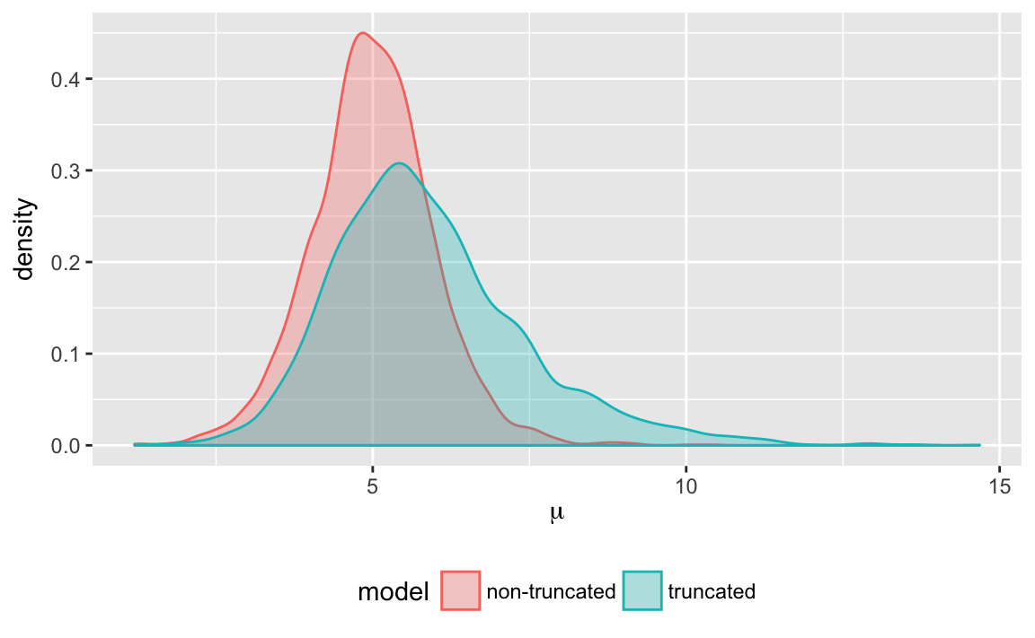
(#fig:truncate_plot_density_mu)Posterior density of $\mu$ when estimated with and without truncation

plot_density("sigma")

$Posterior density of $\sigma$ when estimated with and without truncation$

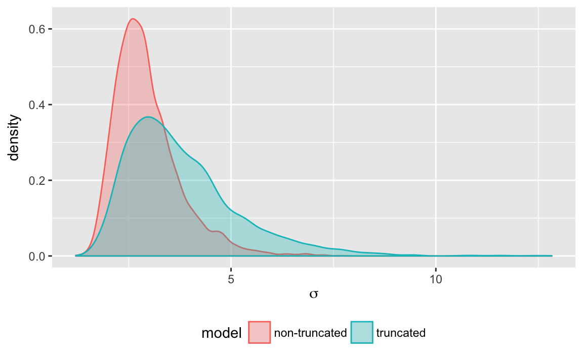
(#fig:truncate_plot_density_sigma)Posterior density of $\sigma$ when estimated with and without truncation

18.3 Questions

How are the densities of $\mu$ and $\sigma$ different under the two models? Why are they different?
Re-estimate the model with improper uniform priors for $\mu$ and $\sigma$. How do the posterior distributions change?
Suppose that the truncation points are unknown. Write a Stan model and estimate. See Stan Development Team (2016), Section 11.2 “Unknown Truncation Points” for how to write such a model. How important is the prior you place on the truncation points?

References

Stan Development Team. 2016. Stan Modeling Language Users Guide and Reference Manual, Version 2.14.0. https://github.com/stan-dev/stan/releases/download/v2.14.0/stan-reference-2.14.0.pdf.

This example is derived from Simon Jackman. “Truncation: How does WinBUGS deal with truncation?” BUGS Examples, 2007-07-24, URL.↩