5 Mississippi Bank Failures in the Great Depression
A difference-in-difference analysis of Mississippi bank failures during the Great Depression (Richardson and Troost 2009). This replicates Figures 5.1–5.3 in Mastering ’Metrics.
library("tidyverse")
library("lubridate")
Load the banks data.
data("banks", package = "masteringmetrics")Only use yearly data in the difference-in-difference estimates. Use the number of banks on July 1st of each year.
banks <- banks %>%
  filter(month(date) == 7L, mday(date) == 1L) %>%
  mutate(year = year(date)) %>%
  select(year, matches("bi[ob][68]"))
Generate the counterfactual using the difference between the number of banks in district 8 and district 6.
banks <- banks %>%
  arrange(year) %>%
  mutate(diff86 = bib8[year == 1930] - bib6[year == 1930],
         counterfactual = if_else(year >= 1930, bib8 - diff86, NA_integer_)) %>%
  select(-diff86)
Plot the lines of the Distinct 8 banks in business, District 6 banks in business, and the District 6 counterfactual. This is equivalent to Figure 5.3 of Angrist and Pischke (2014).
select(banks, year, bib8, bib6, counterfactual) %>%
  gather(variable, value, -year, na.rm = TRUE) %>%
  mutate(variable = recode(variable, bib8 = "8th district",
                           bib6 = "6th district",
                           counterfactual = "Counterfactual")) %>%
  ggplot(aes(x = year, y = value, colour = variable)) +
  geom_point() +
  geom_line() +
  ylab("Number of Banks in Business") +
  xlab("")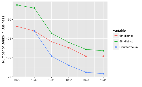
Plot the difference-in-difference estimate for all years after 1930.
ggplot(filter(banks, year > 1930), aes(x = year, y = bib6 - counterfactual)) +
  geom_point() +
  geom_line() +
  ylab("DID (Number of Banks)") +
  xlab("")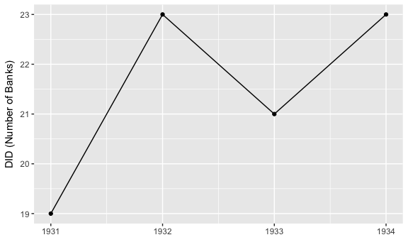
Figure 5.1: Difference between Eighth District and Sixth District Counterfactuals