9 Quarter of Birth and Returns to Schooling
This replicates Tables 6.4 and 6.5, and Figures 6.1 and 6.2 of Mastering ’Metrics. These present an IV analysis of the returns to schooling using quarters of birth (QOB) as instruments for years of schooling (Angrist and Krueger 1991).
library("AER")
library("sandwich")
library("lmtest")
library("tidyverse")
library("broom")
Load twins data.
data("ak91", package = "masteringmetrics")Some cleaning of the data.
ak91 <- mutate(ak91,
               qob_fct = factor(qob),
               q4 = as.integer(qob == "4"),
               yob_fct = factor(yob))
Table 6.4. IV recipe for returns to schooling using a single QOB instrument. Regress log wages on 4th quarter.
mod1 <- lm(lnw ~ q4, data = ak91)
coeftest(mod1, vcov = sandwich)
#>
#> t test of coefficients:
#>
#>             Estimate Std. Error t value Pr(>|t|)
#> (Intercept)  5.89827    0.00136 4329.13   <2e-16 ***
#> q4           0.00681    0.00274    2.48    0.013 *
#> ---
#> Signif. codes:  0 '***' 0.001 '**' 0.01 '*' 0.05 '.' 0.1 ' ' 1
Regress years of schooling on 4th quarter.
mod2 <- lm(s ~ q4, data = ak91)
coeftest(mod2, vcov = sandwich)
#>
#> t test of coefficients:
#>
#>             Estimate Std. Error t value Pr(>|t|)
#> (Intercept) 12.74731    0.00661    1929  < 2e-16 ***
#> q4           0.09212    0.01316       7  2.6e-12 ***
#> ---
#> Signif. codes:  0 '***' 0.001 '**' 0.01 '*' 0.05 '.' 0.1 ' ' 1
IV regression of log wages on years of schooling, with 4th quarter as an instrument for years of schooling.
mod3 <- ivreg(lnw ~ s | q4, data = ak91)
coeftest(mod3, vcov = sandwich)
#>
#> t test of coefficients:
#>
#>             Estimate Std. Error t value Pr(>|t|)
#> (Intercept)    4.955      0.358   13.85   <2e-16 ***
#> s              0.074      0.028    2.64   0.0083 **
#> ---
#> Signif. codes:  0 '***' 0.001 '**' 0.01 '*' 0.05 '.' 0.1 ' ' 1
9.1 Table 6.5
Regression Estimates of Returns to Schooling using Quarter of Birth Instruments
Column 1. OLS
mod4 <- lm(lnw ~ s, data = ak91)
coeftest(mod4, vcov = sandwich)
#>
#> t test of coefficients:
#>
#>             Estimate Std. Error t value Pr(>|t|)
#> (Intercept) 4.995182   0.005074     984   <2e-16 ***
#> s           0.070851   0.000381     186   <2e-16 ***
#> ---
#> Signif. codes:  0 '***' 0.001 '**' 0.01 '*' 0.05 '.' 0.1 ' ' 1
Column 2. IV with only the 4th quarter as an instrument.
mod5 <- ivreg(lnw ~ s | q4, data = ak91)
summary(mod5, vcov = sandwich, diagnostics = TRUE)
#>
#> Call:
#> ivreg(formula = lnw ~ s | q4, data = ak91)
#>
#> Residuals:
#>     Min      1Q  Median      3Q     Max
#> -8.7765 -0.2393  0.0713  0.3326  4.6536
#>
#> Coefficients:
#>             Estimate Std. Error t value Pr(>|t|)
#> (Intercept)    4.955      0.358   13.85   <2e-16 ***
#> s              0.074      0.028    2.64   0.0083 **
#>
#> Diagnostic tests:
#>                     df1    df2 statistic p-value
#> Weak instruments      1 329507     48.99 2.6e-12 ***
#> Wu-Hausman            1 329506      0.01    0.91
#> Sargan                0     NA        NA      NA
#> ---
#> Signif. codes:  0 '***' 0.001 '**' 0.01 '*' 0.05 '.' 0.1 ' ' 1
#>
#> Residual standard error: 0.638 on 329507 degrees of freedom
#> Multiple R-Squared: 0.117,   Adjusted R-squared: 0.117
#> Wald test: 6.97 on 1 and 329507 DF,  p-value: 0.00829
The argument diagnostics = TRUE will run an F-test on the first stage which is reported as the “Weak instruments” diagnostic.
Column 3. OLS. Controls for year of birth.
mod6 <- lm(lnw ~ s + yob_fct, data = ak91)
coeftest(mod6, vcov = sandwich)
#>
#> t test of coefficients:
#>
#>              Estimate Std. Error t value Pr(>|t|)
#> (Intercept)  5.017348   0.006019  833.65  < 2e-16 ***
#> s            0.071081   0.000381  186.34  < 2e-16 ***
#> yob_fct31   -0.006387   0.005123   -1.25  0.21251
#> yob_fct32   -0.014838   0.005052   -2.94  0.00331 **
#> yob_fct33   -0.017583   0.005068   -3.47  0.00052 ***
#> yob_fct34   -0.020999   0.005062   -4.15  3.3e-05 ***
#> yob_fct35   -0.032895   0.005039   -6.53  6.7e-11 ***
#> yob_fct36   -0.031781   0.004970   -6.39  1.6e-10 ***
#> yob_fct37   -0.036712   0.004894   -7.50  6.4e-14 ***
#> yob_fct38   -0.036890   0.004856   -7.60  3.1e-14 ***
#> yob_fct39   -0.048164   0.004833   -9.96  < 2e-16 ***
#> ---
#> Signif. codes:  0 '***' 0.001 '**' 0.01 '*' 0.05 '.' 0.1 ' ' 1
Column 4. IV reg using only the 4th quarter as an instrument. Controls for year of birth.
mod7 <- ivreg(lnw ~ s + yob_fct | q4 + yob_fct, data = ak91)
summary(mod7, vcov = sandwich, diagnostics = TRUE)
#>
#> Call:
#> ivreg(formula = lnw ~ s + yob_fct | q4 + yob_fct, data = ak91)
#>
#> Residuals:
#>     Min      1Q  Median      3Q     Max
#> -8.7785 -0.2346  0.0719  0.3405  4.6687
#>
#> Coefficients:
#>             Estimate Std. Error t value Pr(>|t|)
#> (Intercept)  4.96599    0.35393   14.03   <2e-16 ***
#> s            0.07520    0.02841    2.65   0.0081 **
#> yob_fct31   -0.00696    0.00647   -1.08   0.2819
#> yob_fct32   -0.01557    0.00708   -2.20   0.0279 *
#> yob_fct33   -0.01855    0.00833   -2.23   0.0259 *
#> yob_fct34   -0.02209    0.00909   -2.43   0.0151 *
#> yob_fct35   -0.03425    0.01061   -3.23   0.0012 **
#> yob_fct36   -0.03338    0.01208   -2.76   0.0057 **
#> yob_fct37   -0.03857    0.01368   -2.82   0.0048 **
#> yob_fct38   -0.03910    0.01596   -2.45   0.0143 *
#> yob_fct39   -0.05053    0.01705   -2.96   0.0030 **
#>
#> Diagnostic tests:
#>                     df1    df2 statistic p-value
#> Weak instruments      1 329498     47.73 4.9e-12 ***
#> Wu-Hausman            1 329497      0.02    0.88
#> Sargan                0     NA        NA      NA
#> ---
#> Signif. codes:  0 '***' 0.001 '**' 0.01 '*' 0.05 '.' 0.1 ' ' 1
#>
#> Residual standard error: 0.638 on 329498 degrees of freedom
#> Multiple R-Squared: 0.117,   Adjusted R-squared: 0.117
#> Wald test: 1.81 on 10 and 329498 DF,  p-value: 0.054
Column 4. IV reg using all quarters as instruments. Controls for year of birth.
mod8 <- ivreg(lnw ~ s + yob_fct | qob_fct + yob_fct, data = ak91)
summary(mod8, vcov = sandwich, diagnostics = TRUE)
#>
#> Call:
#> ivreg(formula = lnw ~ s + yob_fct | qob_fct + yob_fct, data = ak91)
#>
#> Residuals:
#>     Min      1Q  Median      3Q     Max
#> -8.9945 -0.2544  0.0676  0.3509  4.8425
#>
#> Coefficients:
#>             Estimate Std. Error t value Pr(>|t|)
#> (Intercept)  4.59174    0.25057   18.32  < 2e-16 ***
#> s            0.10525    0.02012    5.23  1.7e-07 ***
#> yob_fct31   -0.01111    0.00591   -1.88  0.05988 .
#> yob_fct32   -0.02089    0.00623   -3.35  0.00080 ***
#> yob_fct33   -0.02556    0.00698   -3.66  0.00025 ***
#> yob_fct34   -0.03007    0.00742   -4.05  5.1e-05 ***
#> yob_fct35   -0.04414    0.00836   -5.28  1.3e-07 ***
#> yob_fct36   -0.04501    0.00930   -4.84  1.3e-06 ***
#> yob_fct37   -0.05207    0.01034   -5.04  4.7e-07 ***
#> yob_fct38   -0.05518    0.01184   -4.66  3.1e-06 ***
#> yob_fct39   -0.06780    0.01259   -5.39  7.2e-08 ***
#>
#> Diagnostic tests:
#>                     df1    df2 statistic p-value
#> Weak instruments      3 329496     32.32  <2e-16 ***
#> Wu-Hausman            1 329497      2.98   0.084 .
#> Sargan                2     NA      3.26   0.196
#> ---
#> Signif. codes:  0 '***' 0.001 '**' 0.01 '*' 0.05 '.' 0.1 ' ' 1
#>
#> Residual standard error: 0.647 on 329498 degrees of freedom
#> Multiple R-Squared: 0.0905,  Adjusted R-squared: 0.0905
#> Wald test: 3.79 on 10 and 329498 DF,  p-value: 3.9e-05
9.2 Figures
Summarize the average wages by age:
ak91_age <- ak91 %>%
  group_by(qob, yob) %>%
  summarise(lnw = mean(lnw), s = mean(s)) %>%
  mutate(q4 = (qob == 4))
Average years of schooling by quarter of birth for men born in 1930-39 in the 1980 US Census.
ggplot(ak91_age, aes(x = yob + (qob - 1) / 4, y = s)) +
  geom_line() +
  geom_label(mapping = aes(label = qob, color = q4)) +
  theme(legend.position = "none") +
  scale_x_continuous("Year of birth", breaks = 1930:1940) +
  scale_y_continuous("Years of Education", breaks = seq(12.2, 13.2, by = 0.2),
                     limits = c(12.2, 13.2))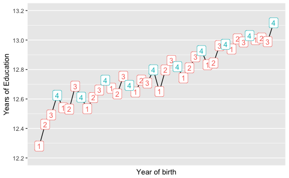
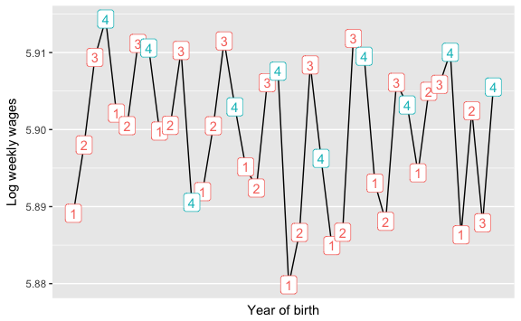
Average log wages by quarter of birth for men born in 1930-39 in the 1980 US Census.
ggplot(ak91_age, aes(x = yob + (qob - 1) / 4, y = lnw)) +
  geom_line() +
  geom_label(mapping = aes(label = qob, color = q4)) +
  scale_x_continuous("Year of birth", breaks = 1930:1940) +
  scale_y_continuous("Log weekly wages") +
  theme(legend.position = "none")