2 RAND Health Insurance Experiment (HIE)

This provides code replicates the Tables 1.3 and 1.4 of Angrist and Pischke (2014) which replicate the analyses from the RAND Health Insurance Experiment (Brook et al. 1983,@Aron-DineEinavEtAl2013).

Load necessary libraries.

library("tidyverse")
library("broom")
library("haven")
library("rlang")
library("clubSandwich")

Function to calculate clustered standard errors and return a tidy data frame of the coefficients and standard errors.

cluster_se <- function(mod, cluster, type = "CR2") {
  vcov <- vcovCR(mod, cluster = cluster, type = type)
  coef_test(mod, vcov = vcov) %>%
    rownames_to_column(var = "term") %>%
    as_tibble() %>%
    select(term, estimate = beta, std.error = SE)
}

2.1 Table 1.3

Angrist and Pischke (2014) Table 1.3 presents demographic and baseline health characteristics for subjects of the RAND Health Insurance Experiment (HIE).

Load the rand data.

data("rand_sample", package = "masteringmetrics")

Calculate the number in each plan:

plantypes <- count(rand_sample, plantype)

knitr::kable(plantypes)

plantype	n
Catastrophic	759
Deductible	881
Coinsurance	1022
Free	1295

For each variable variables, estimate the the difference in means between heath insurance plan types.

varlist <- c("female", "blackhisp", "age", "educper",
             "income1cpi", "hosp", "ghindx", "cholest", "diastol",
             "systol", "mhi", "ghindxx",
             "cholestx", "diastolx", "systolx", "mhix")

Create column (1) with the mean and standard deviation of the “Catastrophic” plan,

catastrophic_stats <- rand_sample %>%
  filter(plantype == "Catastrophic") %>%
  select(one_of(varlist)) %>%
  gather(variable, value) %>%
  group_by(variable) %>%
  summarise(Mean = mean(value, na.rm = TRUE),
            `Std. Dev.` = sd(value, na.rm = TRUE))

knitr::kable(catastrophic_stats, digits = 3)

variable	Mean	Std. Dev.
age	3.24e+01	1.29e+01
blackhisp	1.72e-01	3.77e-01
cholest	2.07e+02	3.99e+01
cholestx	2.03e+02	4.21e+01
diastol	7.48e+01	1.10e+01
diastolx	7.88e+01	1.20e+01
educper	1.21e+01	2.88e+00
female	5.60e-01	4.97e-01
ghindx	7.09e+01	1.49e+01
ghindxx	6.85e+01	1.59e+01
hosp	1.15e-01	3.20e-01
income1cpi	3.16e+04	1.81e+04
mhi	7.38e+01	1.43e+01
mhix	7.55e+01	1.48e+01
systol	1.22e+02	1.65e+01
systolx	1.22e+02	1.87e+01

The difference in means between plans and the catastophic plan.

calc_diffs <- function(x) {
  # programmatically create the formula for lm
  f <- quo(!!sym(x) ~ plantype)
  mod <- lm(f, data = rand_sample)  # nolint
  out <- cluster_se(mod, cluster = rand_sample[["fam_identifier"]])
  out[["response"]] <- x
  out
}

plantype_diffs <- map_dfr(varlist, calc_diffs) %>%
  select(response, term, estimate, std.error) %>%
  mutate(term = str_replace(term, "^plantype", ""))

Create a table similar to Angrist and Pischke (2014) Table 1.3.

fmt_num <- function(x) {
  prettyNum(x, digits = 3, format = "f", big.mark = ",", drop0trailing = FALSE)
}

plantype_diffs %>%
  mutate(estimate = str_c(fmt_num(estimate), " (", fmt_num(std.error), ")")) %>%
  select(-std.error) %>%
  spread(term, estimate) %>%
  knitr::kable(digits = 3)

response	(Intercept)	Coinsurance	Deductible	Free
age	32.4 (0.485)	0.966 (0.655)	0.561 (0.676)	0.435 (0.614)
blackhisp	0.172 (0.0199)	-0.0269 (0.025)	-0.0188 (0.0266)	-0.0281 (0.0245)
cholest	207 (1.99)	-1.93 (2.76)	-1.42 (2.99)	-5.25 (2.7)
cholestx	203 (1.87)	-2.31 (2.47)	0.691 (2.58)	-1.83 (2.39)
diastol	74.8 (0.569)	-0.514 (0.786)	1.22 (0.831)	-0.143 (0.721)
diastolx	78.8 (0.466)	-0.335 (0.617)	0.219 (0.648)	-1.03 (0.588)
educper	12.1 (0.14)	-0.0613 (0.186)	-0.157 (0.191)	-0.263 (0.183)
female	0.56 (0.0118)	-0.0247 (0.0153)	-0.0231 (0.016)	-0.0379 (0.015)
ghindx	70.9 (0.694)	0.211 (0.922)	-1.44 (0.952)	-1.31 (0.872)
ghindxx	68.5 (0.702)	0.612 (0.903)	-0.869 (0.964)	-0.776 (0.867)
hosp	0.115 (0.0117)	-0.00249 (0.0152)	0.00449 (0.016)	0.00117 (0.0146)
income1cpi	31,603 (1,073)	970 (1,391)	-2,104 (1,386)	-976 (1,346)
mhi	73.8 (0.619)	1.19 (0.81)	-0.12 (0.822)	0.89 (0.766)
mhix	75.5 (0.696)	1.07 (0.872)	0.454 (0.911)	0.433 (0.826)
systol	122 (0.805)	0.907 (1.08)	2.32 (1.16)	1.12 (1.01)
systolx	122 (0.782)	-1.39 (0.986)	1.17 (1.06)	-0.522 (0.934)

Plot the difference-in-means of each plantype vs. catastrophic insurance.

ggplot(filter(plantype_diffs, term != "(Intercept)"),
              aes(x = term, y = estimate,
                  ymin = estimate - 2 * std.error,
                  ymax = estimate + 2 * std.error)) +
  geom_hline(yintercept = 0, colour = "white", size = 1) +
  geom_pointrange() +
  facet_grid(response ~ ., scales = "free_y")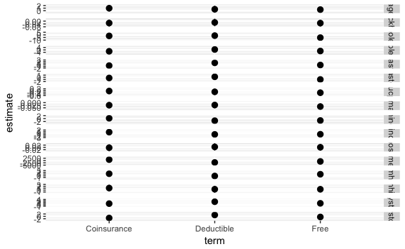

2.2 Table 1.4

Replicate Angrist and Pischke (2014) Table 1.4 which presents health outcome and health expenditure results from the RAND HIE.

data("rand_person_spend", package = "masteringmetrics")

Correlate year variable from annual expenditures data to correct calendar year in order to adjust for inflation.

rand_person_spend <- mutate(rand_person_spend,
                            expyear = indv_start_year + year - 1)

Adjust spending for inflation. The CPI adjustment values below are based on the June CPI from 1991 (see table found at http://www.seattle.gov/financedepartment/cpi/historical.htm).

cpi <- tribble(
  ~ year, ~ cpi,
  1973, 3.07,
  1974, 2.76,
  1975, 2.53,
  1976, 2.39,
  1977, 2.24,
  1978, 2.09,
  1979, 1.88,
  1980, 1.65,
  1981, 1.5,
  1982, 1.41,
  1983, 1.37,
  1984, 1.31,
  1985, 1.27
)

rand_person_spend <- left_join(rand_person_spend,
                               cpi, by = c("expyear" = "year")) %>%
  mutate(out_inf = outsum * cpi,
         inpdol_inf = inpdol * cpi)

Add a total spending variable.

rand_person_spend <- mutate(rand_person_spend,
                       tot_inf = inpdol_inf + out_inf)

Add a variable for any health insurance (free, Individual deductible, or cost-sharing):

rand_person_spend <- mutate(rand_person_spend,
                            any_ins = plantype != "Catastrophic")

Count the number of observations in each plan-type,

count(rand_person_spend, plantype)
#> # A tibble: 4 x 2
#>   plantype         n
#>   <fct>        <int>
#> 1 Catastrophic  3724
#> 2 Deductible    4175
#> 3 Cost Sharing  5464
#> 4 Free          6840

and any-insurance,

count(rand_person_spend, any_ins)
#> # A tibble: 2 x 2
#>   any_ins     n
#>   <lgl>   <int>
#> 1 FALSE    3724
#> 2 TRUE    16479

Create a list of response variables.

varlist <- c("ftf", "out_inf", "totadm", "inpdol_inf", "tot_inf")

Calculate the mean and standard deviation for those receiving catastrophic insurance.

rand_person_spend %>%
  filter(plantype == "Catastrophic") %>%
  select(one_of(varlist)) %>%
  gather(response, value) %>%
  group_by(response) %>%
  summarise(Mean = mean(value, na.rm = TRUE),
            `Std. Dev.` = sd(value, na.rm = TRUE))
#> # A tibble: 5 x 3
#>   response       Mean `Std. Dev.`
#>   <chr>         <dbl>       <dbl>
#> 1 ftf          2.78         5.50 
#> 2 inpdol_inf 388.        2308.   
#> 3 out_inf    248.         488.   
#> 4 tot_inf    636.        2535.   
#> 5 totadm       0.0991       0.379

Calculate the difference in means between plans and the catastophic plan.

calc_diffs <- function(x) {
  # programmatically create the formula
  f <- quo(!!sym(x) ~ plantype)

  mod <- lm(f, data = rand_person_spend)  # nolint
  out <- cluster_se(mod, cluster = rand_person_spend[["fam_identifier"]])
  out[["response"]] <- x
  out
}

person_diffs <- map_dfr(varlist, calc_diffs) %>%
  select(response, term, estimate, std.error) %>%
  mutate(term = str_replace(term, "^plantype", ""))

Standard errors are clustered by family identifier using the clubSandwich package.

Print the table. If this were an actual publication, I’d make it nicer.

fmt_num <- function(x) {
  prettyNum(x, digits = 3, format = "f", big.mark = ",", drop0trailing = FALSE)
}

person_diffs %>%
  mutate(estimate = str_c(fmt_num(estimate), " (", fmt_num(std.error), ")")) %>%
  select(-std.error) %>%
  spread(term, estimate) %>%
  knitr::kable(digits = 3)

response	(Intercept)	Cost Sharing	Deductible	Free
ftf	2.78 (0.178)	0.481 (0.24)	0.193 (0.247)	1.66 (0.248)
inpdol_inf	388 (44.9)	92.5 (72.8)	72.2 (68.6)	116 (59.8)
out_inf	248 (14.8)	59.8 (20.7)	41.8 (20.8)	169 (19.9)
tot_inf	636 (54.5)	152 (84.6)	114 (79.1)	285 (72.4)
totadm	0.0991 (0.00785)	0.0023 (0.0108)	0.0159 (0.0109)	0.0288 (0.0105)

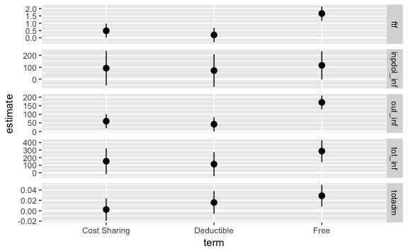
Additionally we could plot the difference-in-means of each plan type vs. catastrophic insurance.

ggplot(filter(person_diffs, term != "(Intercept)"),
              aes(x = term, y = estimate,
                  ymin = estimate - 2 * std.error,
                  ymax = estimate + 2 * std.error)) +
  geom_hline(yintercept = 0, colour = "white", size = 1) +
  geom_pointrange() +
  facet_grid(response ~ ., scales = "free_y")

References

• https://www.icpsr.umich.edu/icpsrweb/NACDA/studies/6439/version/1
• http://masteringmetrics.com/wp-content/uploads/2015/01/ReadMe_RAND.txt
• http://masteringmetrics.com/wp-content/uploads/2015/01/Code.zip