2 Causality
Prerequisites
library("tidyverse")
library("stringr")
2.1 Racial Discrimination in the Labor Market
Load the data from the qss package.
data("resume", package = "qss")In addition to the dim(), summary(), and head() functions shown in the text,
dim(resume)
#> [1] 4870    4
summary(resume)
#>   firstname             sex                race                call
#>  Length:4870        Length:4870        Length:4870        Min.   :0.00
#>  Class :character   Class :character   Class :character   1st Qu.:0.00
#>  Mode  :character   Mode  :character   Mode  :character   Median :0.00
#>                                                           Mean   :0.08
#>                                                           3rd Qu.:0.00
#>                                                           Max.   :1.00
head(resume)
#>   firstname    sex  race call
#> 1   Allison female white    0
#> 2   Kristen female white    0
#> 3   Lakisha female black    0
#> 4   Latonya female black    0
#> 5    Carrie female white    0
#> 6       Jay   male white    0
we can also use glimpse() to get a quick understanding of the variables in the data frame:
glimpse(resume)
#> Observations: 4,870
#> Variables: 4
#> $ firstname <chr> "Allison", "Kristen", "Lakisha", "Latonya", "Carrie"...
#> $ sex       <chr> "female", "female", "female", "female", "female", "m...
#> $ race      <chr> "white", "white", "black", "black", "white", "white"...
#> $ call      <int> 0, 0, 0, 0, 0, 0, 0, 0, 0, 0, 0, 0, 0, 0, 0, 0, 0, 0...
The code in QSS uses table() and addmargins() to construct the table. However, this can be done easily with the dplyr package using grouping and summarizing.
Use group_by() to identify each combination of race and call, and then count() the observations:
race_call_tab <-
  resume %>%
  group_by(race, call) %>%
  count()
race_call_tab
#> # A tibble: 4 x 3
#> # Groups:   race, call [4]
#>   race   call     n
#>   <chr> <int> <int>
#> 1 black     0  2278
#> 2 black     1   157
#> 3 white     0  2200
#> 4 white     1   235
If we want to calculate callback rates by race, we can use the mutate() function from dplyr.
race_call_rate <-
  race_call_tab %>%
  group_by(race) %>%
  mutate(call_rate =  n / sum(n)) %>%
  filter(call == 1) %>%
  select(race, call_rate)
race_call_rate
#> # A tibble: 2 x 2
#> # Groups:   race [2]
#>   race  call_rate
#>   <chr>     <dbl>
#> 1 black    0.0645
#> 2 white    0.0965
If we want the overall callback rate, we can calculate it from the original data. Use the summarise() function from dplyr.
resume %>%
  summarise(call_back = mean(call))
#>   call_back
#> 1    0.0805
2.2 Subsetting Data in R
2.2.1 Subsetting
Create a new object of all individuals whose race variable equals black in the resume data:
resumeB <-
  resume %>%
filter(race == "black")glimpse(resumeB)
#> Observations: 2,435
#> Variables: 4
#> $ firstname <chr> "Lakisha", "Latonya", "Kenya", "Latonya", "Tyrone", ...
#> $ sex <chr> "female", "female", "female", "female", "male", "fem...
#> $ race <chr> "black", "black", "black", "black", "black", "black"...
#> $ call <int> 0, 0, 0, 0, 0, 0, 0, 0, 0, 0, 0, 0, 0, 0, 0, 0, 0, 0...Calculate the callback rate for black individuals:
resumeB %>%
  summarise(call_rate = mean(call))
#>   call_rate
#> 1    0.0645
You can combine the filter() and select() functions with multiple conditions. For example, to keep the call and first name variables for female individuals with stereotypically black names:
resumeBf <-
  resume %>%
  filter(race == "black", sex == "female") %>%
  select(call, firstname)
head(resumeBf)
#>   call firstname
#> 1    0   Lakisha
#> 2    0   Latonya
#> 3    0     Kenya
#> 4    0   Latonya
#> 5    0     Aisha
#> 6    0     Aisha
Now we can calculate the gender gap by group.
Now we can calculate the gender gap by group. Doing so may seem to require a little more code, but we will not duplicate as much as in QSS, and this would easily scale to more than two categories.
First, group by race and sex and calculate the callback rate for each group:
resume_race_sex <-
  resume %>%
  group_by(race, sex) %>%
  summarise(call = mean(call))
head(resume_race_sex)
#> # A tibble: 4 x 3
#> # Groups:   race [2]
#>   race  sex      call
#>   <chr> <chr>   <dbl>
#> 1 black female 0.0663
#> 2 black male   0.0583
#> 3 white female 0.0989
#> 4 white male   0.0887
Use spread() from the tidyr package to make each value of race a new column:
resume_sex <-
  resume_race_sex %>%
  ungroup() %>%
  spread(race, call)
resume_sex
#> # A tibble: 2 x 3
#>   sex     black  white
#>   <chr>   <dbl>  <dbl>
#> 1 female 0.0663 0.0989
#> 2 male   0.0583 0.0887
Now we can calculate the race wage differences by sex as before,
resume_sex %>%
  mutate(call_diff = white - black)
#> # A tibble: 2 x 4
#>   sex     black  white call_diff
#>   <chr>   <dbl>  <dbl>     <dbl>
#> 1 female 0.0663 0.0989    0.0326
#> 2 male   0.0583 0.0887    0.0304
This could be combined into a single chain with only six lines of code:
resume %>%
  group_by(race, sex) %>%
  summarise(call = mean(call)) %>%
  ungroup() %>%
  spread(race, call) %>%
  mutate(call_diff = white - black)
#> # A tibble: 2 x 4
#>   sex     black  white call_diff
#>   <chr>   <dbl>  <dbl>     <dbl>
#> 1 female 0.0663 0.0989    0.0326
#> 2 male   0.0583 0.0887    0.0304
For more information on a way to do this using the spread and gather functions from tidyr package, see the R for Data Science chapter “Tidy Data”.
WARNING The function ungroup removes the groupings in group_by. The function spread will not allow a grouping variable to be reshaped. Since many dplyr functions work differently depending on whether the data frame is grouped or not, I find that I can encounter many errors due to forgetting that a data frame is grouped. As such, I tend to ungroup data frames as soon as I am no longer are using the groupings.
Alternatively, we could have used summarise and the diff function:
resume %>%
  group_by(race, sex) %>%
  summarise(call = mean(call)) %>%
  group_by(sex) %>%
  arrange(race) %>%
  summarise(call_diff = diff(call))
#> # A tibble: 2 x 2
#>   sex    call_diff
#>   <chr>      <dbl>
#> 1 female    0.0326
#> 2 male      0.0304
I find the spread code preferable since the individual race callback rates are retained in the data, and since there is no natural ordering of the race variable (unlike if it were a time-series), it is not obvious from reading the code whether call_diff is black - white or white - black.
2.2.2 Simple conditional statements
dlpyr has three conditional statement functions if_else, recode and case_when.
The function if_else is like ifelse but corrects inconsistent behavior that ifelse exhibits in certain cases.
Create a variable BlackFemale using if_else() and confirm it is only equal to 1 for black and female observations:
resume %>%
  mutate(BlackFemale = if_else(race == "black" & sex == "female", 1, 0)) %>%
  group_by(BlackFemale, race, sex) %>%
  count()
#> # A tibble: 4 x 4
#> # Groups:   BlackFemale, race, sex [4]
#>   BlackFemale race  sex        n
#>         <dbl> <chr> <chr>  <int>
#> 1        0    black male     549
#> 2        0    white female  1860
#> 3        0    white male     575
#> 4        1.00 black female  1886
Warning The function if_else is more strict about the variable types than ifelse. While most R functions are forgiving about variables types, and will automatically convert integers to numeric or vice-versa, they are distinct. For example, these examples will produce errors:
resume %>%
  mutate(BlackFemale = if_else(race == "black" & sex == "female", TRUE, 0))
#> Error in mutate_impl(.data, dots): Evaluation error: `false` must be type logical, not double.
because TRUE is logical and 0 is numeric.
resume %>%
  mutate(BlackFemale = if_else(race == "black" & sex == "female", 1L, 0))
#> Error in mutate_impl(.data, dots): Evaluation error: `false` must be type integer, not double.
because 1L is an integer and 0 is numeric vector (floating-point number). The distinction between integers and numeric variables is often invisible because most functions coerce variables between integer and numeric vectors.
class(1)
#> [1] "numeric"
class(1L)
#> [1] "integer"
The : operator returns integers and as.integer coerces numeric vectors to integer vectors:
class(1:5)
#> [1] "integer"
class(c(1, 2, 3))
#> [1] "numeric"
class(as.integer(c(1, 2, 3)))
#> [1] "integer"
2.2.3 Factor Variables
For more on factors see the R for Data Science chapter “Factors” and the package forcats. Also see the R for Data Science chapter “Strings” for working with strings.
The function case_when is a generalization of the if_else function to multiple conditions. For example, to create categories for all combinations of race and sex,
resume %>%
  mutate(
    race_sex = case_when(
      race == "black" & sex == "female" ~ "black, female",
      race == "white" & sex == "female" ~ "white female",
      race == "black" & sex == "male" ~ "black male",
      race == "white" & sex == "male" ~ "white male"
    )
  ) %>%
  head()
#>   firstname    sex  race call      race_sex
#> 1   Allison female white    0  white female
#> 2   Kristen female white    0  white female
#> 3   Lakisha female black    0 black, female
#> 4   Latonya female black    0 black, female
#> 5    Carrie female white    0  white female
#> 6       Jay   male white    0    white male
Each condition is a formula (an R object created with the “tilde” ~). You will see formulas used extensively in the modeling section. The condition is on the left-hand side of the formula. The value to assign to observations meeting that condition is on the right-hand side. Observations are given the value of the first matching condition, so the order of these can matter.
The case_when function also supports a default value by using a condition TRUE as the last condition. This will match anything not already matched. For example, if you wanted three categories (“black male”, “black female”, “white”):
resume %>%
  mutate(
    race_sex = case_when(
      race == "black" & sex == "female" ~ "black female",
      race == "black" & sex == "male" ~ "black male",
      TRUE ~ "white"
    )
  ) %>%
  head()
#>   firstname    sex  race call     race_sex
#> 1   Allison female white    0        white
#> 2   Kristen female white    0        white
#> 3   Lakisha female black    0 black female
#> 4   Latonya female black    0 black female
#> 5    Carrie female white    0        white
#> 6       Jay   male white    0        white
Alternatively, we could have created this variable using string manipulation functions. Use mutate() to create a new variable, type, str_to_title to capitalize sex and race, and str_c to concatenate these vectors.
resume <-
  resume %>%
  mutate(type = str_c(str_to_title(race), str_to_title(sex)))
Some of the reasons given in QSS for using factors in this chapter are less important due to the functionality of modern tidyverse packages. For example, there is no reason to use tapply, as you can use group_by and summarise,
resume %>%
  group_by(type) %>%
  summarise(call = mean(call))
#> # A tibble: 4 x 2
#>   type          call
#>   <chr>        <dbl>
#> 1 BlackFemale 0.0663
#> 2 BlackMale   0.0583
#> 3 WhiteFemale 0.0989
#> 4 WhiteMale   0.0887
or,
resume %>%
  group_by(race, sex) %>%
  summarise(call = mean(call))
#> # A tibble: 4 x 3
#> # Groups:   race [?]
#>   race  sex      call
#>   <chr> <chr>   <dbl>
#> 1 black female 0.0663
#> 2 black male   0.0583
#> 3 white female 0.0989
#> 4 white male   0.0887
What’s nice about this approach is that we wouldn’t have needed to create the factor variable first as in QSS.
We can use that same approach to calculate the mean of first names, and use arrange() to sort in ascending order.
resume %>%
  group_by(firstname) %>%
  summarise(call = mean(call)) %>%
  arrange(call)
#> # A tibble: 36 x 2
#>   firstname   call
#>   <chr>      <dbl>
#> 1 Aisha     0.0222
#> 2 Rasheed   0.0299
#> 3 Keisha    0.0383
#> 4 Tremayne  0.0435
#> 5 Kareem    0.0469
#> 6 Darnell   0.0476
#> # ... with 30 more rows**Tip:** General advice for working (or not) with factors:
- Use character vectors instead of factors. They are easier to manipulate with string functions.
- Use factor vectors only when you need a specific ordering of string values in a variable, e.g. in a model or a plot.
2.3 Causal Affects and the Counterfactual
Load the social dataset included in the qss package.
data("social", package = "qss")
summary(social)
#>      sex             yearofbirth    primary2004      messages
#>  Length:305866      Min.   :1900   Min.   :0.000   Length:305866
#>  Class :character   1st Qu.:1947   1st Qu.:0.000   Class :character
#>  Mode  :character   Median :1956   Median :0.000   Mode  :character
#>                     Mean   :1956   Mean   :0.401
#>                     3rd Qu.:1965   3rd Qu.:1.000
#>                     Max.   :1986   Max.   :1.000
#>   primary2006        hhsize
#>  Min.   :0.000   Min.   :1.00
#>  1st Qu.:0.000   1st Qu.:2.00
#>  Median :0.000   Median :2.00
#>  Mean   :0.312   Mean   :2.18
#>  3rd Qu.:1.000   3rd Qu.:2.00
#>  Max.   :1.000   Max.   :8.00
Calculate the mean turnout by message:
turnout_by_message <-
  social %>%
  group_by(messages) %>%
  summarize(turnout = mean(primary2006))
turnout_by_message
#> # A tibble: 4 x 2
#>   messages   turnout
#>   <chr>        <dbl>
#> 1 Civic Duty   0.315
#> 2 Control      0.297
#> 3 Hawthorne    0.322
#> 4 Neighbors    0.378
Since we want to calculate the difference by group, spread() the data set so each group is a column, then use mutate() to calculate the difference of each from the control group. Finally, use select() and matches() to return a dataframe with only those new variables that you have created:
turnout_by_message %>%
  spread(messages, turnout) %>%
  mutate(diff_civic_duty = `Civic Duty` - Control,
         diff_Hawthorne = Hawthorne - Control,
         diff_Neighbors = Neighbors - Control) %>%
  select(matches("diff_"))
#> # A tibble: 1 x 3
#>   diff_civic_duty diff_Hawthorne diff_Neighbors
#>             <dbl>          <dbl>          <dbl>
#> 1          0.0179         0.0257         0.0813
Find the mean values of age, 2004 turnout, and household size for each group:
social %>%
  mutate(age = 2006 - yearofbirth) %>%
  group_by(messages) %>%
  summarise(primary2004 = mean(primary2004),
            age = mean(age),
            hhsize = mean(hhsize))
#> # A tibble: 4 x 4
#>   messages   primary2004   age hhsize
#>   <chr>            <dbl> <dbl>  <dbl>
#> 1 Civic Duty       0.399  49.7   2.19
#> 2 Control          0.400  49.8   2.18
#> 3 Hawthorne        0.403  49.7   2.18
#> 4 Neighbors        0.407  49.9   2.19
The function summarise_at allows you to summarize multiple variables, using multiple functions, or both.
social %>%
  mutate(age = 2006 - yearofbirth) %>%
  group_by(messages) %>%
  summarise_at(vars(primary2004, age, hhsize), funs(mean))
#> # A tibble: 4 x 4
#>   messages   primary2004   age hhsize
#>   <chr>            <dbl> <dbl>  <dbl>
#> 1 Civic Duty       0.399  49.7   2.19
#> 2 Control          0.400  49.8   2.18
#> 3 Hawthorne        0.403  49.7   2.18
#> 4 Neighbors        0.407  49.9   2.19
2.4 Observational Studies
Load and inspect the minimum wage data from the qss package:
data("minwage", package = "qss")
glimpse(minwage)
#> Observations: 358
#> Variables: 8
#> $ chain      <chr> "wendys", "wendys", "burgerking", "burgerking", "kf...
#> $ location   <chr> "PA", "PA", "PA", "PA", "PA", "PA", "PA", "PA", "PA...
#> $ wageBefore <dbl> 5.00, 5.50, 5.00, 5.00, 5.25, 5.00, 5.00, 5.00, 5.0...
#> $ wageAfter  <dbl> 5.25, 4.75, 4.75, 5.00, 5.00, 5.00, 4.75, 5.00, 4.5...
#> $ fullBefore <dbl> 20.0, 6.0, 50.0, 10.0, 2.0, 2.0, 2.5, 40.0, 8.0, 10...
#> $ fullAfter  <dbl> 0.0, 28.0, 15.0, 26.0, 3.0, 2.0, 1.0, 9.0, 7.0, 18....
#> $ partBefore <dbl> 20.0, 26.0, 35.0, 17.0, 8.0, 10.0, 20.0, 30.0, 27.0...
#> $ partAfter  <dbl> 36, 3, 18, 9, 12, 9, 25, 32, 39, 10, 20, 4, 13, 20,...
summary(minwage)
#>     chain             location           wageBefore     wageAfter
#>  Length:358         Length:358         Min.   :4.25   Min.   :4.25
#>  Class :character   Class :character   1st Qu.:4.25   1st Qu.:5.05
#>  Mode  :character   Mode  :character   Median :4.50   Median :5.05
#>                                        Mean   :4.62   Mean   :4.99
#>                                        3rd Qu.:4.99   3rd Qu.:5.05
#>                                        Max.   :5.75   Max.   :6.25
#>    fullBefore     fullAfter      partBefore     partAfter
#>  Min.   : 0.0   Min.   : 0.0   Min.   : 0.0   Min.   : 0.0
#>  1st Qu.: 2.1   1st Qu.: 2.0   1st Qu.:11.0   1st Qu.:11.0
#>  Median : 6.0   Median : 6.0   Median :16.2   Median :17.0
#>  Mean   : 8.5   Mean   : 8.4   Mean   :18.8   Mean   :18.7
#>  3rd Qu.:12.0   3rd Qu.:12.0   3rd Qu.:25.0   3rd Qu.:25.0
#>  Max.   :60.0   Max.   :40.0   Max.   :60.0   Max.   :60.0
First, calculate the proportion of restaurants by state whose hourly wages were less than the minimum wage in NJ, $5.05, for wageBefore and wageAfter:
Since the NJ minimum wage was $5.05, we’ll define a variable with that value. Even if you use them only once or twice, it is a good idea to put values like this in variables. It makes your code closer to self-documenting, i.e. easier for others (including you, in the future) to understand what the code does.
NJ_MINWAGE <- 5.05Later, it will be easier to understand wageAfter < NJ_MINWAGE without any comments than it would be to understand wageAfter < 5.05. In the latter case you’d have to remember that the new NJ minimum wage was 5.05 and that’s why you were using that value. Using 5.05 in your code, instead of assigning it to an object called NJ_MINWAGE, is an example of a magic number; try to avoid them.
Note that the variable location has multiple values: PA and four regions of NJ. So we’ll add a state variable to the data.
minwage %>%
  count(location)
#> # A tibble: 5 x 2
#>   location      n
#>   <chr>     <int>
#> 1 centralNJ    45
#> 2 northNJ     146
#> 3 PA           67
#> 4 shoreNJ      33
#> 5 southNJ      67
We can extract the state from the final two characters of the location variable using thestringr function str_sub:
minwage <-
  mutate(minwage, state = str_sub(location, -2L))
Alternatively, since "PA" is the only value that an observation in Pennsylvania takes in location, and since all other observations are in New Jersey:
minwage <-
  mutate(minwage, state = if_else(location == "PA", "PA", "NJ"))
Let’s confirm that the restaurants followed the law:
minwage %>%
  group_by(state) %>%
  summarise(prop_after = mean(wageAfter < NJ_MINWAGE),
            prop_Before = mean(wageBefore < NJ_MINWAGE))
#> # A tibble: 2 x 3
#>   state prop_after prop_Before
#>   <chr>      <dbl>       <dbl>
#> 1 NJ       0.00344       0.911
#> 2 PA       0.955         0.940
Create a variable for the proportion of full-time employees in NJ and PA after the increase:
minwage <-
  minwage %>%
  mutate(totalAfter = fullAfter + partAfter,
        fullPropAfter = fullAfter / totalAfter)
Now calculate the average proportion of full-time employees for each state:
full_prop_by_state <-
  minwage %>%
  group_by(state) %>%
  summarise(fullPropAfter = mean(fullPropAfter))
full_prop_by_state
#> # A tibble: 2 x 2
#>   state fullPropAfter
#>   <chr>         <dbl>
#> 1 NJ            0.320
#> 2 PA            0.272
We could compute the difference in means between NJ and PA by
(filter(full_prop_by_state, state == "NJ")[["fullPropAfter"]] -
  filter(full_prop_by_state, state == "PA")[["fullPropAfter"]])
#> [1] 0.0481
or
spread(full_prop_by_state, state, fullPropAfter) %>%
  mutate(diff = NJ - PA)
#> # A tibble: 1 x 3
#>      NJ    PA   diff
#>   <dbl> <dbl>  <dbl>
#> 1 0.320 0.272 0.0481
2.4.1 Confounding Bias
We can calculate the proportion of each chain out of all fast-food restaurants in each state:
chains_by_state <-
  minwage %>%
  group_by(state) %>%
  count(chain) %>%
  mutate(prop = n / sum(n))
We can easily compare these using a dot-plot:
ggplot(chains_by_state, aes(x = chain, y = prop, colour = state)) +
  geom_point() +
  coord_flip()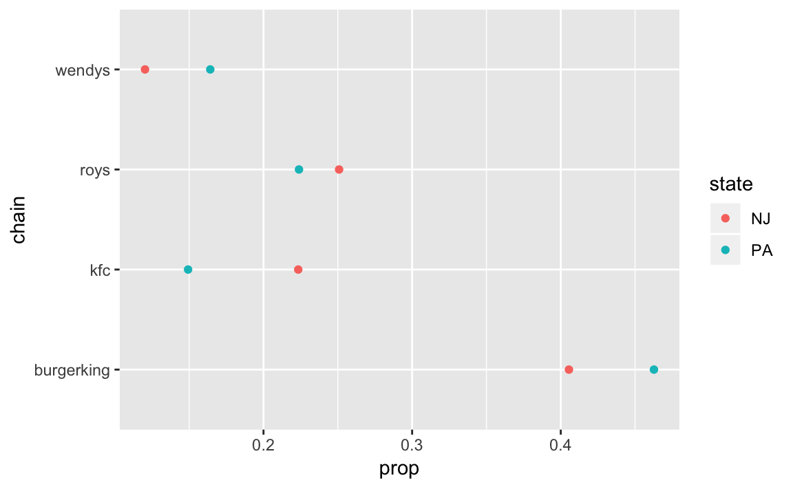
In the QSS text, only Burger King restaurants are compared. However, dplyr makes comparing all restaurants not much more complicated than comparing two. All we have to do is change the group_by statement we used previously so that we group by chain restaurants and states:
full_prop_by_state_chain <-
  minwage %>%
  group_by(state, chain) %>%
  summarise(fullPropAfter = mean(fullPropAfter))
full_prop_by_state_chain
#> # A tibble: 8 x 3
#> # Groups:   state [?]
#>   state chain      fullPropAfter
#>   <chr> <chr>              <dbl>
#> 1 NJ    burgerking         0.358
#> 2 NJ    kfc                0.328
#> 3 NJ    roys               0.283
#> 4 NJ    wendys             0.260
#> 5 PA    burgerking         0.321
#> 6 PA    kfc                0.236
#> # ... with 2 more rows
We can plot and compare the proportions easily in this format. In general, ordering categorical variables alphabetically is useless, so we’ll order the chains by the average of the NJ and PA fullPropAfter, using fct_reorder function:
ggplot(full_prop_by_state_chain,
       aes(x = forcats::fct_reorder(chain, fullPropAfter),
           y = fullPropAfter,
           colour = state)) +
  geom_point() +
  coord_flip() +
  labs(x = "chains")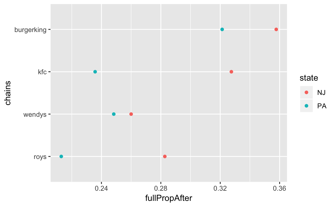
To calculate the difference between states in the proportion of full-time employees after the change:
full_prop_by_state_chain %>%
  spread(state, fullPropAfter) %>%
  mutate(diff = NJ - PA)
#> # A tibble: 4 x 4
#>   chain         NJ    PA   diff
#>   <chr>      <dbl> <dbl>  <dbl>
#> 1 burgerking 0.358 0.321 0.0364
#> 2 kfc        0.328 0.236 0.0918
#> 3 roys       0.283 0.213 0.0697
#> 4 wendys     0.260 0.248 0.0117
2.4.2 Before and After and Difference-in-Difference Designs
To compute the estimates in the before and after design first create an additional variable for the proportion of full-time employees before the minimum wage increase.
minwage <-
  minwage %>%
  mutate(totalBefore = fullBefore + partBefore,
         fullPropBefore = fullBefore / totalBefore)
The before-and-after analysis is the difference between the full-time employment before and after the minimum wage law passed looking only at NJ:
minwage %>%
  filter(state == "NJ") %>%
  summarise(diff = mean(fullPropAfter) - mean(fullPropBefore))
#>     diff
#> 1 0.0239
The difference-in-differences design uses the difference in the before-and-after differences for each state.
minwage %>%
  group_by(state) %>%
  summarise(diff = mean(fullPropAfter) - mean(fullPropBefore)) %>%
  spread(state, diff) %>%
  mutate(diff_in_diff = NJ - PA)
#> # A tibble: 1 x 3
#>       NJ      PA diff_in_diff
#>    <dbl>   <dbl>        <dbl>
#> 1 0.0239 -0.0377       0.0616
Let’s create a single dataset with the mean values of each state before and after to visually look at each of these designs:
full_prop_by_state <-
  minwage %>%
  group_by(state) %>%
  summarise_at(vars(fullPropAfter, fullPropBefore), mean) %>%
  gather(period, fullProp, -state) %>%
  mutate(period = recode(period, fullPropAfter = 1, fullPropBefore = 0))
full_prop_by_state
#> # A tibble: 4 x 3
#>   state period fullProp
#>   <chr>  <dbl>    <dbl>
#> 1 NJ         1    0.320
#> 2 PA         1    0.272
#> 3 NJ         0    0.297
#> 4 PA         0    0.310
Now plot this new dataset:
ggplot(full_prop_by_state, aes(x = period, y = fullProp, colour = state)) +
  geom_point() +
  geom_line() +
  scale_x_continuous(breaks = c(0, 1), labels = c("Before", "After"))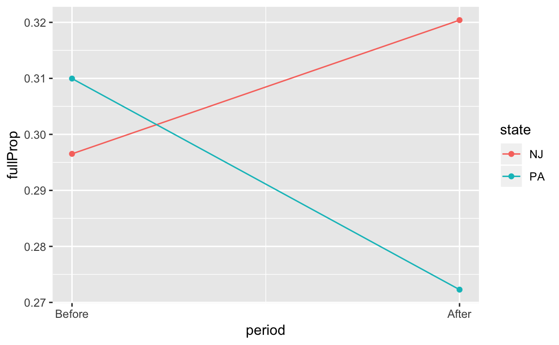
2.5 Descriptive Statistics for a Single Variable
To calculate the summary for the variables wageBefore and wageAfter for New Jersey only:
minwage %>%
  filter(state == "NJ") %>%
  select(wageBefore, wageAfter) %>%
  summary()
#>    wageBefore     wageAfter
#>  Min.   :4.25   Min.   :5.00
#>  1st Qu.:4.25   1st Qu.:5.05
#>  Median :4.50   Median :5.05
#>  Mean   :4.61   Mean   :5.08
#>  3rd Qu.:4.87   3rd Qu.:5.05
#>  Max.   :5.75   Max.   :5.75
We calculate the interquartile range for each state’s wages after the passage of the law using the same grouped summarize as we used before:
minwage %>%
  group_by(state) %>%
  summarise(wageAfter = IQR(wageAfter),
            wageBefore = IQR(wageBefore))
#> # A tibble: 2 x 3
#>   state wageAfter wageBefore
#>   <chr>     <dbl>      <dbl>
#> 1 NJ        0           0.62
#> 2 PA        0.575       0.75
Calculate the variance and standard deviation of wageAfter and wageBefore for each state:
minwage %>%
  group_by(state) %>%
  summarise(wageAfter_sd = sd(wageAfter),
               wageAfter_var = var(wageAfter),
               wageBefore_sd = sd(wageBefore),
               wageBefore_var = var(wageBefore))
#> # A tibble: 2 x 5
#>   state wageAfter_sd wageAfter_var wageBefore_sd wageBefore_var
#>   <chr>        <dbl>         <dbl>         <dbl>          <dbl>
#> 1 NJ           0.106        0.0112         0.343          0.118
#> 2 PA           0.359        0.129          0.358          0.128
Here we can see again how using summarise_at allows for more compact code to specify variables and summary statistics that would be the case using just summarise:
minwage %>%
  group_by(state) %>%
  summarise_at(vars(wageAfter, wageBefore), funs(sd, var))
#> # A tibble: 2 x 5
#>   state wageAfter_sd wageBefore_sd wageAfter_var wageBefore_var
#>   <chr>        <dbl>         <dbl>         <dbl>          <dbl>
#> 1 NJ           0.106         0.343        0.0112          0.118
#> 2 PA           0.359         0.358        0.129           0.128