6 Probability

Prerequisites

library("tidyverse")
library("forcats")
library("stringr")
library("broom")

6.1 Probability

6.1.1 Frequentist vs. Bayesian

6.1.2 Definition and Axioms

6.1.3 Permutations

birthday <- function(k) {
  logdenom <- k * log(365) + lfactorial(365 - k)
  lognumer <- lfactorial(365)
  pr <- 1 -   exp(lognumer - logdenom)
  pr
}

bday <- tibble(k = 1:50, pr = birthday(k))

ggplot(bday, aes(x = k, y = pr)) +
  geom_hline(yintercept = 0.5, colour = "white", size = 2) +
  geom_line() +
  geom_point() +
  scale_y_continuous(str_c("Probability that at least two",
                           "people have the same birthday", sep = "\n"),
                     limits = c(0, 1), breaks = seq(0, 1, by = 0.1)) +
  labs(x = "Number of people")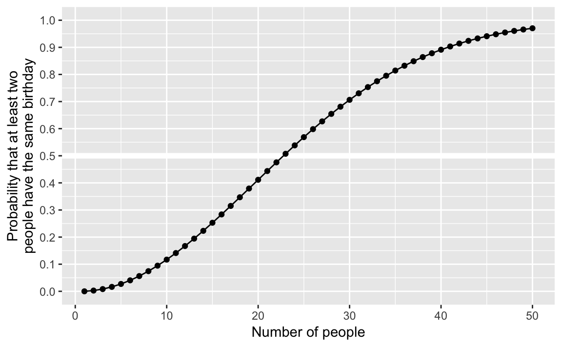

Note: The logarithm is used for numerical stability. Basically, “floating-point” numbers are approximations of numbers. If you perform arithmetic with numbers that are very large, very small, or vary differently in magnitudes, you could have problems. Logarithms help with some of those issues. See “Falling Into the Floating Point Trap” in The R Inferno for a summary of floating point numbers. See these John Fox posts 1 2 for an example of numerical stability gone wrong. Also see this article on the log sum of exponentials.

6.1.4 Sampling without replacement

Instead of using a for loop, we could do the simulations using a functional as described in R for Data Science chapter “Iterations”.

Define the function sim_bdays which randomly samples k birthdays, and returns TRUE if there are any duplicate birthdays, and FALSE if there are none.

sim_bdays <- function(k) {
  days <- sample(1:365, k, replace = TRUE)
  length(unique(days)) < k
}

We can test the code for k = 10 birthdays.

sim_bdays(10)
#> [1] FALSE

Since the function is randomly sampling birthdays, running it multiple times will produce different answers.

One helpful feature of a functional style of writing code vs. a for loop is that the function encapsulates the code and allows you to test that it works for different inputs before repeating it for many inputs. It is more difficult to debug functions that produce random outputs, but some sanity checks are that the function:

returns a logical vector of length one (TRUE or FALSE)
always returns FALSE when k = 1 since there can never be a duplicates with one person
always returns TRUE when k > 365 by the pidgeonhole principle.

sim_bdays(1)
#> [1] FALSE
sim_bdays(366)
#> [1] TRUE

Set the parameters for 1,000 simulations, and 23 individuals. We use map_lgl since sim_bdays returns a logical value (TRUE, FALSE):

sims <- 1000
k <- 23
map_lgl(seq_len(sims), ~ sim_bdays(k)) %>%
  mean()
#> [1] 0.489

An alternative way of running this is using the rerun and using flatten to turn the output to a numeric vector:

rerun(sims, sim_bdays(k)) %>%
  flatten_dbl() %>%
  mean()
#> [1] 0.477

6.1.5 Combinations

The function for \(84\choose{6}\) is:

choose(84, 6)
#> [1] 4.06e+08

However, due to the the larges values that the binomial coefficient, it is almost always better to use the log of the binomial coefficient, \(\log{84\choose{6}}\),

lchoose(84, 6)
#> [1] 19.8

6.2 Conditional Probability

6.2.1 Conditional, Marginal, and Joint Probabilities

Load Florida voting data from the qss package:

data(FLVoters, package = "qss")
dim(FLVoters)
#> [1] 10000     6
glimpse(FLVoters)
#> Observations: 10,000
#> Variables: 6
#> $ surname <chr> "PIEDRA", "LYNCH", "CHESTER", "LATHROP", "HUMMEL", "CH...
#> $ county  <int> 115, 115, 115, 115, 115, 115, 115, 115, 1, 1, 115, 115...
#> $ VTD     <int> 66, 13, 103, 80, 8, 55, 84, 48, 41, 39, 26, 45, 11, 48...
#> $ age     <int> 58, 51, 63, 54, 77, 49, 77, 34, 56, 60, 44, 45, 80, 83...
#> $ gender  <chr> "f", "m", "m", "m", "f", "m", "f", "f", "f", "m", "m",...
#> $ race    <chr> "white", "white", NA, "white", "white", "white", "whit...
FLVoters <- FLVoters %>%
  na.omit()
dim(FLVoters)
#> [1] 9113    6

Note the difference between glimpse() and dim(). What is different in how they handle NA observations?

Instead of using prop.base, we calculate the probabilities with a data frame. Calculate the marginal probabilities of each race:

margin_race <-
  FLVoters %>%
  count(race) %>%
  mutate(prop = n / sum(n))
margin_race
#> # A tibble: 6 x 3
#>   race         n    prop
#>   <chr>    <int>   <dbl>
#> 1 asian      175 0.0192 
#> 2 black     1194 0.131  
#> 3 hispanic  1192 0.131  
#> 4 native      29 0.00318
#> 5 other      310 0.0340 
#> 6 white     6213 0.682

Calculate the marginal probabilities of each gender:

margin_gender <-
  FLVoters %>%
  count(gender) %>%
  mutate(prop = n / sum(n))
margin_gender
#> # A tibble: 2 x 3
#>   gender     n  prop
#>   <chr>  <int> <dbl>
#> 1 f       4883 0.536
#> 2 m       4230 0.464

FLVoters %>%
  filter(gender == "f") %>%
  count(race) %>%
  mutate(prop = n / sum(n))
#> # A tibble: 6 x 3
#>   race         n    prop
#>   <chr>    <int>   <dbl>
#> 1 asian       83 0.0170 
#> 2 black      678 0.139  
#> 3 hispanic   666 0.136  
#> 4 native      17 0.00348
#> 5 other      158 0.0324 
#> 6 white     3281 0.672

joint_p <-
  FLVoters %>%
  count(gender, race) %>%
  mutate(prop = n / sum(n))
joint_p
#> # A tibble: 12 x 4
#>   gender race         n    prop
#>   <chr>  <chr>    <int>   <dbl>
#> 1 f      asian       83 0.00911
#> 2 f      black      678 0.0744 
#> 3 f      hispanic   666 0.0731 
#> 4 f      native      17 0.00187
#> 5 f      other      158 0.0173 
#> 6 f      white     3281 0.360  
#> # ... with 6 more rows

We can convert the data frame to have gender as columns:

joint_p %>%
  select(-n) %>%
  spread(gender, prop)
#> # A tibble: 6 x 3
#>   race           f       m
#>   <chr>      <dbl>   <dbl>
#> 1 asian    0.00911 0.0101 
#> 2 black    0.0744  0.0566 
#> 3 hispanic 0.0731  0.0577 
#> 4 native   0.00187 0.00132
#> 5 other    0.0173  0.0167 
#> 6 white    0.360   0.322

Sum over race:

joint_p %>%
  group_by(race) %>%
  summarise(prop = sum(prop))
#> # A tibble: 6 x 2
#>   race        prop
#>   <chr>      <dbl>
#> 1 asian    0.0192 
#> 2 black    0.131  
#> 3 hispanic 0.131  
#> 4 native   0.00318
#> 5 other    0.0340 
#> 6 white    0.682

Sum over gender:

joint_p %>%
  group_by(gender) %>%
  summarise(prop = sum(prop))
#> # A tibble: 2 x 2
#>   gender  prop
#>   <chr>  <dbl>
#> 1 f      0.536
#> 2 m      0.464

FLVoters <-
  FLVoters %>%
  mutate(age_group = cut(age, c(0, 20, 40, 60, Inf), right = TRUE,
                         labels = c("<= 20", "20-40", "40-60", "> 60")))

joint3 <-
  FLVoters %>%
  count(race, age_group, gender) %>%
  ungroup() %>%
  mutate(prop = n / sum(n))
joint3
#> # A tibble: 47 x 5
#>   race  age_group gender     n     prop
#>   <chr> <fct>     <chr>  <int>    <dbl>
#> 1 asian <= 20     f          1 0.000110
#> 2 asian <= 20     m          2 0.000219
#> 3 asian 20-40     f         24 0.00263 
#> 4 asian 20-40     m         26 0.00285 
#> 5 asian 40-60     f         38 0.00417 
#> 6 asian 40-60     m         47 0.00516 
#> # ... with 41 more rows

Marginal probabilities by age groups

margin_age <-
  FLVoters %>%
  count(age_group) %>%
  mutate(prop = n / sum(n))
margin_age
#> # A tibble: 4 x 3
#>   age_group     n   prop
#>   <fct>     <int>  <dbl>
#> 1 <= 20       161 0.0177
#> 2 20-40      2469 0.271 
#> 3 40-60      3285 0.360 
#> 4 > 60       3198 0.351

Calculate the probabilities that each group is in a given age group, and show \(P(\text{black} \land \text{female} \land \text{age} > 60)\): (Note: the symbol \(\land\) is the logical symbol for ‘and’, implying the joint probability.)

left_join(joint3,
          select(margin_age, age_group, margin_age = prop),
          by = "age_group") %>%
  mutate(prob_age_group = prop / margin_age) %>%
  filter(race == "black", gender == "f", age_group == "> 60") %>%
  select(race, age_group, gender, prob_age_group)
#> # A tibble: 1 x 4
#>   race  age_group gender prob_age_group
#>   <chr> <fct>     <chr>           <dbl>
#> 1 black > 60      f              0.0538

Two-way joint probability table for age group and gender

joint2 <- FLVoters %>%
  count(age_group, gender) %>%
  ungroup() %>%
  mutate(prob_age_gender = n / sum(n))
joint2
#> # A tibble: 8 x 4
#>   age_group gender     n prob_age_gender
#>   <fct>     <chr>  <int>           <dbl>
#> 1 <= 20     f         88         0.00966
#> 2 <= 20     m         73         0.00801
#> 3 20-40     f       1304         0.143  
#> 4 20-40     m       1165         0.128  
#> 5 40-60     f       1730         0.190  
#> 6 40-60     m       1555         0.171  
#> # ... with 2 more rows

The joint probability \(P(\text{age} > 60 \land \text{female})\),

joint2 %>%
  filter(age_group == "> 60", gender == "f")
#> # A tibble: 1 x 4
#>   age_group gender     n prob_age_gender
#>   <fct>     <chr>  <int>           <dbl>
#> 1 > 60      f       1761           0.193

The conditional probabilities \(P(\text{race } | \text{ gender, age})\),

condprob_race <-
  left_join(joint3, select(joint2, -n), by = c("age_group", "gender")) %>%
  mutate(prob_race = prop / prob_age_gender) %>%
  arrange(age_group, gender) %>%
  select(age_group, gender, race, prob_race)

Each row is the \(P(\text{race } | \text{ age group} \land \text{gender})\), so \(P(\text{black } | \text{ female} \land \text{age} > 60)\),

filter(condprob_race, gender == "f", age_group == "> 60", race == "black")
#> # A tibble: 1 x 4
#>   age_group gender race  prob_race
#>   <fct>     <chr>  <chr>     <dbl>
#> 1 > 60      f      black    0.0977

6.2.2 Independence

Create a table with the products of margins of race and age. Using the function crossing to create a tibble with all combinations of race and gender and the independent prob.

race_gender_indep <-
  crossing(select(margin_race, race, prob_race = prop),
           select(margin_gender, gender, prob_gender = prop)) %>%
  mutate(prob_indep = prob_race * prob_gender) %>%
  left_join(select(joint_p, gender, race, prob = prop),
            by = c("gender", "race")) %>%
  select(race, gender, everything())
race_gender_indep
#> # A tibble: 12 x 6
#>   race     gender prob_race prob_gender prob_indep    prob
#>   <chr>    <chr>      <dbl>       <dbl>      <dbl>   <dbl>
#> 1 asian    f         0.0192       0.536    0.0103  0.00911
#> 2 asian    m         0.0192       0.464    0.00891 0.0101 
#> 3 black    f         0.131        0.536    0.0702  0.0744 
#> 4 black    m         0.131        0.464    0.0608  0.0566 
#> 5 hispanic f         0.131        0.536    0.0701  0.0731 
#> 6 hispanic m         0.131        0.464    0.0607  0.0577 
#> # ... with 6 more rows

ggplot(race_gender_indep,
       aes(x = prob_indep, y = prob, colour = race)) +
  geom_abline(intercept = 0, slope = 1, colour = "white", size = 2) +
  geom_point() +
  facet_grid(. ~ gender) +
  coord_fixed() +
  theme(legend.position = "bottom") +
  labs(x = expression(P("race") * P("gender")),
       y = expression(P("race and gender")))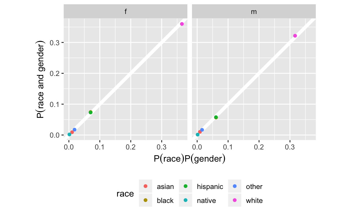

While the original code only calculates joint-independence value for values of age > 60, and female, this calculates the joint probabilities for all combinations of the three variables, and facets by age and gender.

joint_indep <-
  crossing(select(margin_race, race, prob_race = prop),
           select(margin_age, age_group, prob_age = prop),
           select(margin_gender, gender, prob_gender = prop)) %>%
  mutate(indep_prob = prob_race * prob_age * prob_gender) %>%
  left_join(select(joint3, race, age_group, gender, prob = prop),
            by = c("gender", "age_group", "race")) %>%
  replace_na(list(prob = 0))

ggplot(joint_indep, aes(x = prob, y = indep_prob, colour = race)) +
  geom_abline(intercept = 0, slope = 1, colour = "white", size = 2) +
  geom_point() +
  facet_grid(age_group ~ gender) +
  coord_fixed() +
  labs(x = "P(race and age and gender)",
       y = "P(race) * P(age) * P(gender)",
       title = "Joint Independence")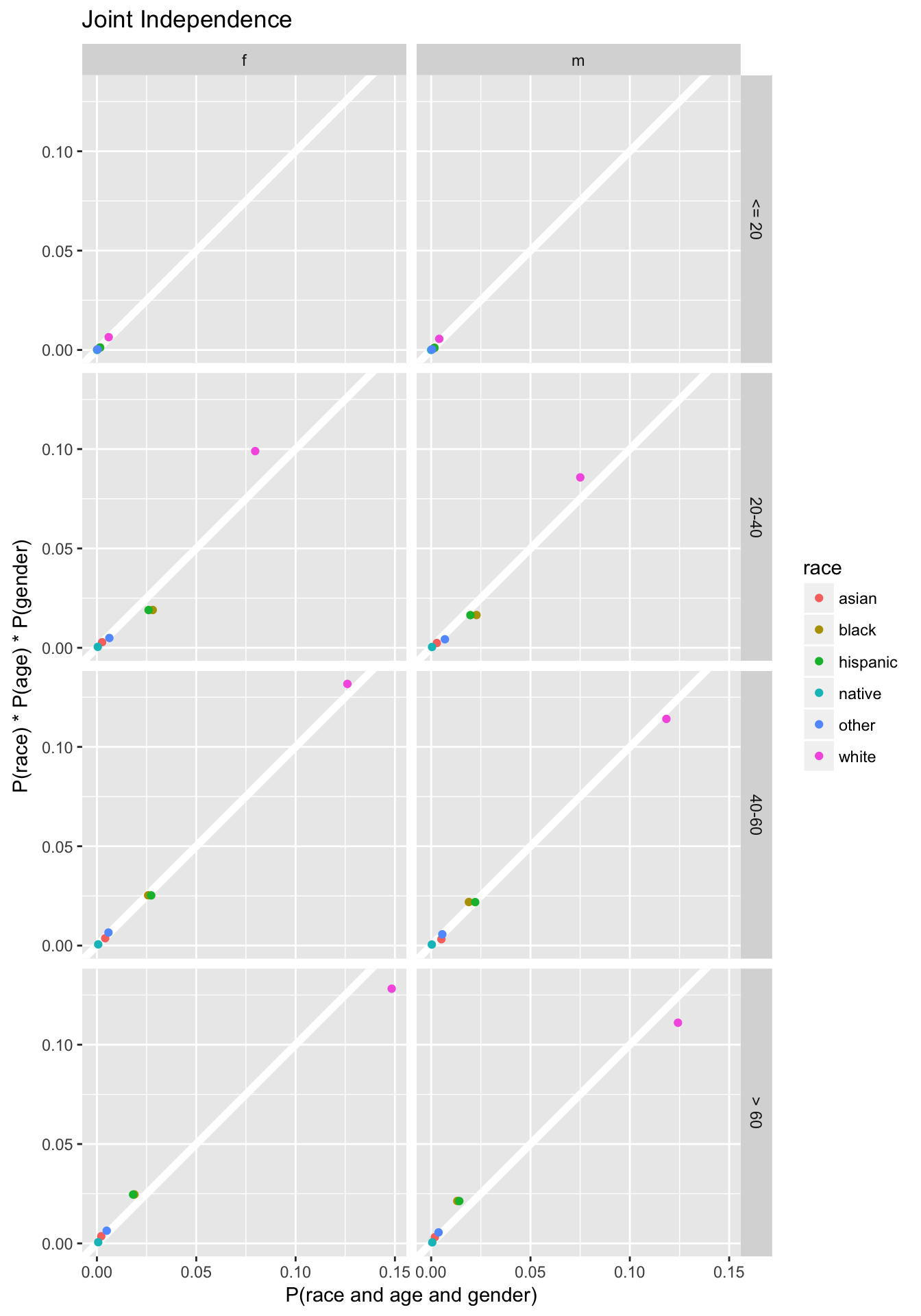

While code in QSS only calculates the conditional independence given female, the following code calculates conditional independence for all values of gender:

cond_gender <-
  left_join(select(joint3, race, age_group, gender, joint_prob = prop),
            select(margin_gender, gender, prob_gender = prop),
            by = c("gender")) %>%
  mutate(cond_prob = joint_prob / prob_gender)

Calculate the conditional distribution \(\Pr(\text{race} | \text{gender})\):

prob_race_gender <-
  left_join(select(joint_p, race, gender, prob_race_gender = prop),
            select(margin_gender, gender, prob_gender = prop),
            by = "gender") %>%
  mutate(prob_race = prob_race_gender / prob_gender)

Calculate the conditional distribution \(\Pr(\text{age} | \text{gender})\):

prob_age_gender <-
  left_join(select(joint2, age_group, gender, prob_age_gender),
            select(margin_gender, gender, prob_gender = prop),
            by = "gender") %>%
  mutate(prob_age = prob_age_gender / prob_gender)

# indep prob of race and age
indep_cond_gender <-
  full_join(select(prob_race_gender, race, gender, prob_race),
            select(prob_age_gender, age_group, gender, prob_age),
            by = "gender") %>%
  mutate(indep_prob = prob_race * prob_age)

inner_join(select(indep_cond_gender, race, age_group, gender, indep_prob),
           select(cond_gender, race, age_group, gender, cond_prob),
           by = c("gender", "age_group", "race")) %>%
  ggplot(aes(x = cond_prob, y = indep_prob, colour = race)) +
  geom_abline(intercept = 0, slope = 1, colour = "white", size = 2) +
  geom_point() +
  facet_grid(age_group ~ gender) +
  coord_fixed() +
  labs(x = "P(race and age | gender)",
       y = "P(race | gender) * P(age | gender)",
       title = "Marginal independence")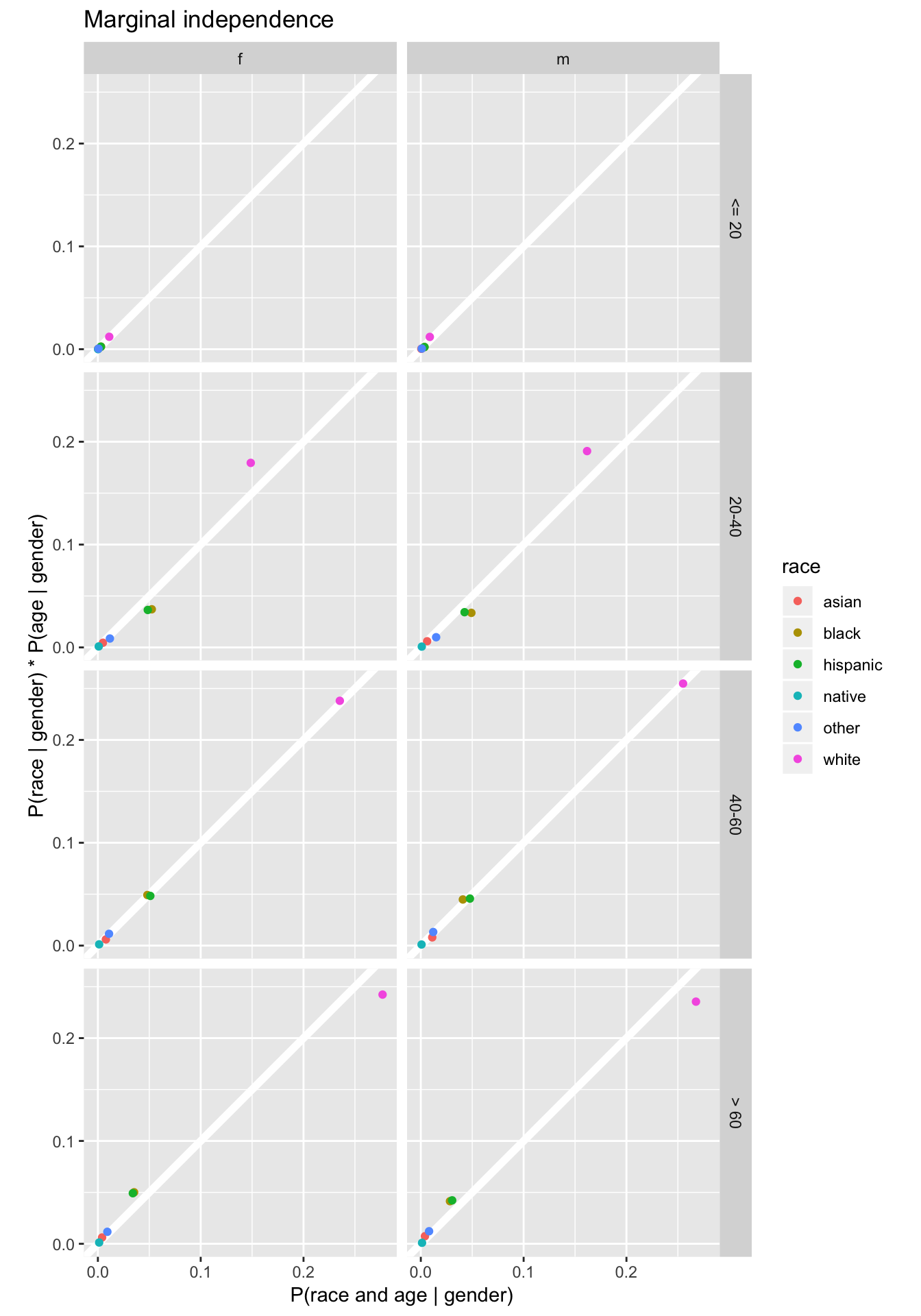

6.2.2.1 Monty-hall problem

The for loop approach in QSS is valid code, but here we provide a more functional approach to solving the problem. We will define a function to choose a door, repeat the function multiple times while storing the results in a data frame, and then summarize that data frame.

First, create a function for a single iteration. This returns a single logical value:

choose_door <- function(.iter) {
  # what's behind each door door:
  # Why is it okay that this is fixed?
  doors <- c("goat", "goat", "car")

  # User randomly chooses a door
  first <- sample(1:3, 1)

  # randomly choose the door that Monty Hall reveals
  remain <- doors[-first]
  monty <- sample( (1:2)[remain == "goat"], size = 1)
  # did the contestant win?
  tibble(.iter = .iter,
         result = remain[-monty] == "car")
}

Now use map_df to run choose_door multiple times, and then summarize the results:

sims <- 1000
map_df(seq_len(sims), choose_door) %>%
  summarise(win_pct = mean(result))
#> # A tibble: 1 x 1
#>   win_pct
#>     <dbl>
#> 1   0.648

6.2.3 Bayes’ Rule

6.2.4 Predicting Race Using Surname and Residence Location

Start with the Census names files:

data("cnames", package = "qss")
glimpse(cnames)
#> Observations: 151,671
#> Variables: 7
#> $ surname     <chr> "SMITH", "JOHNSON", "WILLIAMS", "BROWN", "JONES", ...
#> $ count       <int> 2376206, 1857160, 1534042, 1380145, 1362755, 11278...
#> $ pctwhite    <dbl> 73.34, 61.55, 48.52, 60.72, 57.69, 85.80, 64.73, 6...
#> $ pctblack    <dbl> 22.22, 33.80, 46.72, 34.54, 37.73, 10.41, 30.77, 0...
#> $ pctapi      <dbl> 0.40, 0.42, 0.37, 0.41, 0.35, 0.42, 0.40, 1.43, 0....
#> $ pcthispanic <dbl> 1.56, 1.50, 1.60, 1.64, 1.44, 1.43, 1.58, 90.82, 9...
#> $ pctothers   <dbl> 2.48, 2.73, 2.79, 2.69, 2.79, 1.94, 2.52, 1.09, 0....

For each surname, cnames contains variables with the probability that it belongs to an individual of a given race (pctwhite, pctblack, …). We want to find the most-likely race for a given surname, by finding the race with the maximum proportion. Instead of dealing with multiple variables, it is easier to use max on a single variable, so we will rearrange the data to in order to use a grouped summarize, and then merge the new variable back to the original data sets. We will also remove the ‘pct’ prefix from each of the variable names.

Calculate the most likely race for each name:

most_likely_race <-
  cnames %>%
  select(-count) %>%
  gather(race_pred, pct, -surname) %>%
  # remove pct_ prefix from variable names
  mutate(race_pred = str_replace(race_pred, "^pct", "")) %>%
  # # group by surname
  group_by(surname) %>%
  # select obs with the largest percentage
  filter(row_number(desc(pct)) == 1L) %>%
  # Ungroup to avoid errors later
  ungroup %>%
  # # don't need pct anymore
  select(-pct) %>%
  mutate(race_pred = recode(race_pred, asian = "api", other = "others"))

Merge the data frame with the most likely race for each surname to the the original cnames data frame:

cnames <-
  cnames %>%
  left_join(most_likely_race, by = "surname")

Instead of using match, use inner_join to merge the surnames to FLVoters:

FLVoters <-
  FLVoters %>%
  inner_join(cnames, by = "surname")
dim(FLVoters)
#> [1] 8022   14

FLVoters also includes a “native” category that the surname dataset does not.

FLVoters <-
  FLVoters %>%
  mutate(race2 = fct_recode(race, other = "native"))

Check that the levels of race and race_pred are the same:

FLVoters %>%
  count(race2)
#> # A tibble: 5 x 2
#>   race2        n
#>   <fct>    <int>
#> 1 asian      140
#> 2 black     1078
#> 3 hispanic  1023
#> 4 other      277
#> 5 white     5504
FLVoters %>%
  count(race_pred)
#> # A tibble: 5 x 2
#>   race_pred     n
#>   <chr>     <int>
#> 1 api         120
#> 2 black       258
#> 3 hispanic   1121
#> 4 others        7
#> 5 white      6516

Now we can calculate True positive rate for all races

FLVoters %>%
  group_by(race2) %>%
  summarise(tp = mean(race2 == race_pred)) %>%
  arrange(desc(tp))
#> # A tibble: 5 x 2
#>   race2       tp
#>   <fct>    <dbl>
#> 1 white    0.950
#> 2 hispanic 0.847
#> 3 black    0.160
#> 4 asian    0    
#> 5 other    0

and the False discovery rate for all races,

FLVoters %>%
  group_by(race_pred) %>%
  summarise(fp = mean(race2 != race_pred)) %>%
  arrange(desc(fp))
#> # A tibble: 5 x 2
#>   race_pred    fp
#>   <chr>     <dbl>
#> 1 api       1    
#> 2 others    1    
#> 3 black     0.329
#> 4 hispanic  0.227
#> 5 white     0.197

Now add residence data using the FLCensus data included in the

data("FLCensus", package = "qss")

\(P(\text{race})\) in Florida:

race.prop <-
  FLCensus %>%
  select(total.pop, white, black, api, hispanic, others) %>%
  gather(race, pct, -total.pop) %>%
  group_by(race) %>%
  summarise(mean = weighted.mean(pct, weights = total.pop)) %>%
  arrange(desc(mean))
race.prop
#> # A tibble: 5 x 2
#>   race       mean
#>   <chr>     <dbl>
#> 1 white    0.605 
#> 2 hispanic 0.213 
#> 3 black    0.139 
#> 4 api      0.0219
#> 5 others   0.0214

6.2.5 Predicting Election Outcomes with Uncertainty

Load the pres08 data from the qss package.

data("pres08", package = "qss")

Add a column p which contains Obama’s vote share of the major parties:

pres08 <- pres08 %>%
  mutate(p = Obama / (Obama + McCain))

Write a function to simulate the elections. df is the data frame (pres08) with the state, EV, and p columns. n_draws is the size of the binomial distribution to draw from. .id is the simulation number.

sim_election <- function(.id, df, n_draws = 1000) {
  # For each state randomly sample
  mutate(df,
         draws = rbinom(n(), n_draws, p)) %>%
  filter(draws > (n_draws / 2)) %>%
  summarise(EV = sum(EV),
            .id = .id)
}

Now simulate the election 10,000 times:

sims <- 10000
sim_results <- map_df(seq_len(sims), ~ sim_election(.x, pres08, n_draws = 1000))

In the 2008 election, Obama received 364 electoral votes

ELECTION_EV <- 364

And plot them,

ggplot(sim_results, aes(x = EV, y = ..density..)) +
  geom_histogram(binwidth = 10, fill = "gray30") +
  geom_vline(xintercept = ELECTION_EV, colour = "black", size = 2) +
  labs(x = "Electoral Votes", y = "density")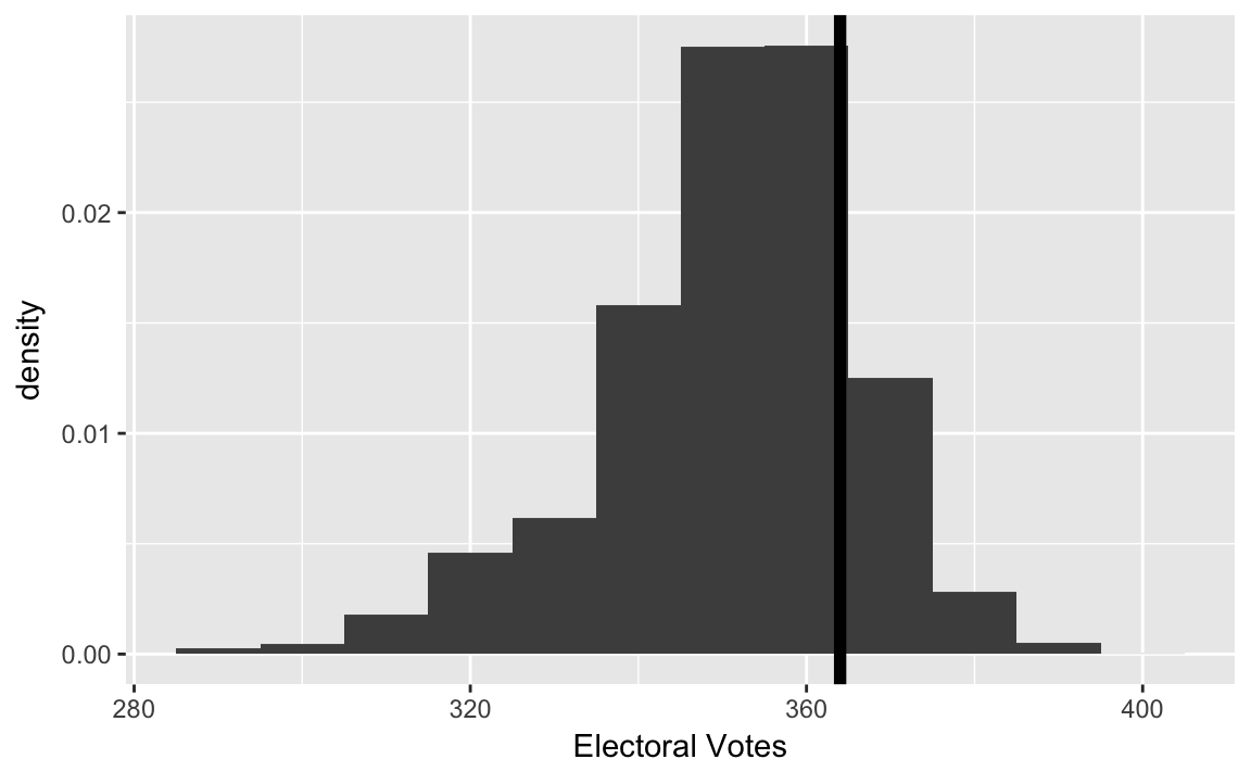

Simulation mean, variance, and standard deviations:

sim_results %>%
  select(EV) %>%
  summarise_all(funs(mean, var, sd))
#>   mean var   sd
#> 1  352 269 16.4

Theoretical probabilities from a binomial distribution:

# we cannot use n, because mutate will look for n() first.
n_draws <- 1000
pres08 %>%
  mutate(pb = pbinom(n_draws / 2, size = n_draws, prob = p,
                     lower.tail  = FALSE)) %>%
  summarise(mean = sum(pb * EV),
            V = sum(pb * (1 - pb) * EV ^ 2),
            sd = sqrt(V))
#>   mean   V   sd
#> 1  352 269 16.4

6.3 Random Variables and Probability Distributions

6.3.1 Bernoulli and Uniform Distributions

Uniform distribution functions:

dunif(0.5, min = 0, max = 1)
#> [1] 1
punif(1, min = -2, max = 2)
#> [1] 0.75

Sample from a uniform distribution, and convert to a probability:

sims <- 1000
p <- 0.5

A Bernoulli distribution is a discrete distribution which randomly samples from 0 and 1. A random variable \(X\) with a Bernoulli distribution with probability parameter \(p\) has the distribution, \[ \begin{aligned} P(X = 1 | p) &= p \\ P(X = 0 | p) &= 1 - p \end{aligned} \]

R does not have a rbernoulli for the Bernoulli distribution (because as we will see it is a special case of the Binomial distribution, and there are several other ways to sample from it): Here are three ways to sample from a Bernoulli distribution.

First, we can use the sample from values c(0, 1) with replacement. By default it will set sample 0 and 1 with equal probability (\(p = 0.5\)), but using the prob argument we can sample 0 and 1 with difference probabilities. Take 50 samples from a Bernoulli distribution with p = 0.6,

p <- 0.6
n <- 100
y <- sample(c(0, 1), n, prob = c(1 - p, p), replace = TRUE)
head(y)
#> [1] 1 0 1 1 1 1
mean(y)
#> [1] 0.57

A second method to sample \(n\) values from a Bernoulli distribution that has a probability parameter \(p\) is,

Take a sample of \(n\) values from a uniform distribution. Call this vector \(x\).
To generate a sample \(y\) taking values of 0 and 1 from this vector \(x\), set \(y_i = 1\) if \(x_i >= p\), and \(y_i = 0\) if \(x_i < p\).

Note how this method works. Given a value \(p\) between 0 and 1, in a sample from Uniform distribution, in expectation a fraction of \(p\) values will be less than \(p\), and in expectation a fraction of \(1 - p\) values will be greater than \(p\). These are exactly the probabilities of sampling 1 and 0 in the probability mass of the Uniform distribution: {r} y <- as.integer(runif(n, min = 0, max = 1) <= p) head(y) mean(y)ß

Third, note that the Bernoulli distribution is a special case of the binomial distribution (discussed in the next section), where \(size = 1\). Thus, we can use the rbinom function to sample from a binomial distribution.

y <- rbinom(n, size = 1, prob = p)
head(y)
#> [1] 1 1 1 0 1 1
mean(y)
#> [1] 0.64

Since the R functions for the Binomial distribution don’t exist here are examples of how you would write them as examples of writing functions to sample and calculate the PDF or PMF, CDF, and quantile functions of a distribution. Sample from the distribution:

rbernoulli <- function(n, prob = 0.5) {
  sample(c(1L, 0L), n, replace = FALSE, prob = c(prob, 1 - prob))
}

Probability mass function (PMF):

dbernoulli <- function(x, prob = 0.5) {
  d <- rep(NA_real_, length(x))
  d[x == 1] <- prob
  d[x == 0] <- 1 - prob
  d
}

Cumulative density function (CDF): \[ P(X \leq x|p) = \begin{cases} 0 & \text{if } x < 0 , \\ 1 - p & \text{if } 0 \leq x < 1 ,\\ 1 & \text{if } x \geq 1 . \end{cases} \]

pbernoulli <- function(q, prob = 0.5) {
  p <- rep(NA_real_, length(q))
  p[q < 0] <- 0
  p[q >= 0 & q < 1] <- 1 - prob
  p[q >= 1] <- 1
  p
}

The inverse cumulative density function or quantile function, \[ q = \begin{cases} \emptyset & \text{if } x \leq 1 - p, \\ 0 & \text{if } 1 - p \leq x < 1 ,\\ 1 & \text{if } x \geq 1 . \end{cases} \] where, \[ q \text{ such that } P(X \leq q|p) = x. \]

qbernoulli <- function(p, prob = 0.5) {
  q <- rep(NA_integer_, length(p))
  q[prob >= 1 - p & prob < 1] <- 0L
  q[prob >= 1] <- 1L
  q
}

Alternatively, since the Bernoulli distribution is a special case of the Binomial distribution, write *bernoulli functions that wrap calls to to *binom functions for the special case where size = 1:

rbernoulli <- function(n, prob = 0.5, ...) {
  rbinom(n, size = 1, prob = prob, ...)
}
pbernoulli <- function(q, prob = 0.5, ...) {
  rbinom(q, size = 1, prob = prob, ...)
}
pbernoulli <- function(q, prob = 0.5, ...) {
  rbinom(q, size = 1, prob = prob, ...)
}
dbernoulli <- function(x, prob = 0.5, ...) {
  rbinom(x, size = 1, prob = prob, ...)
}

6.3.2 Binomial distribution

dbinom(2, size = 3, prob = 0.5)
#> [1] 0.375
pbinom(1, 3, 0.5)
#> [1] 0.5

voters <- c(1000, 10000, 100000)
dbinom(voters / 2, size = voters, prob = 0.5)
#> [1] 0.02523 0.00798 0.00252

6.3.3 Normal distribution

pnorm(1) - pnorm(-1)
#> [1] 0.683
pnorm(2) - pnorm(-2)
#> [1] 0.954

Write a function to calculate the area of a normal distribution \(\pm \sigma\)

normal_pm_sigma <- function(x, mu = 0, sd = 1) {
  (pnorm(mu + sd * x, mean = mu, sd = sd) -
     pnorm(mu - sd * x, mean = mu, sd = sd))
}
normal_pm_sigma(1)
#> [1] 0.683
normal_pm_sigma(2)
#> [1] 0.954
normal_pm_sigma(1, mu = 5, sd = 2)
#> [1] 0.683
normal_pm_sigma(2, mu = 5, sd = 2)
#> [1] 0.954

data("pres08", package = "qss")
data("pres12", package = "qss")

To join both data frames

pres <-
  full_join(select(pres08, state, Obama_2008 = Obama, McCain_2008 = McCain,
                 EV_2008 = EV),
          select(pres12, state, Obama_2012 = Obama, Romney_2012 = Romney,
                 EV_2012 = EV),
          by = "state") %>%
  mutate(Obama_2008_z = as.numeric(scale(Obama_2008)),
         Obama_2012_z = as.numeric(scale(Obama_2012)))

fit1 <- lm(Obama_2012_z ~ -1 + Obama_2008_z, data = pres)

Plot the residuals and compare them to a normal distribution:

err <- tibble(err = resid(fit1)) %>%
  # z-score of residuals
  mutate(err_std = err / sd(err))

ggplot(err, aes(x = err_std)) +
  geom_histogram(mapping = aes(y = ..density..),
                 binwidth = 1, boundary = 0) +
  stat_function(geom = "line", fun = dnorm) +
  scale_x_continuous("Standardized residuals",
                     breaks = -3:3, limits = c(-3, 3))

ggplot(err, aes(sample = err_std)) +
  geom_abline(intercept = 0, slope = 1, color = "white", size = 2) +
  geom_qq() +
  coord_fixed(ratio = 1) +
  scale_y_continuous("Sample quantiles", limits = c(-3, 3)) +
  scale_x_continuous("Theoretical quantiles", limits = c(-3, 3))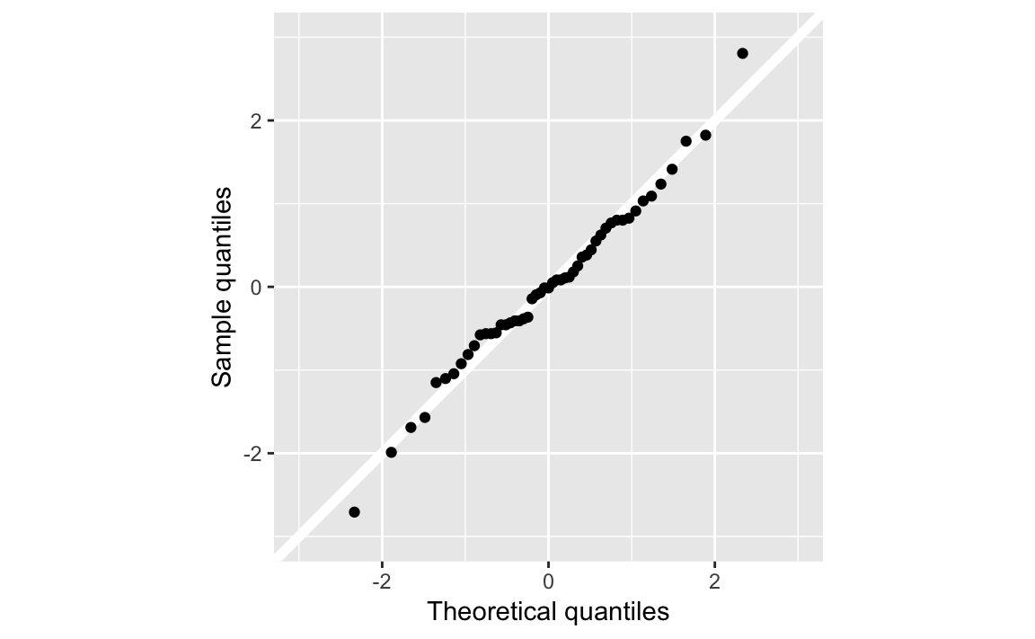

Alternatively, you can use the augment function from broom which returns the residuals for each observation in the .resid column.

augment(fit1) %>%
  mutate(.resid_z = .resid / sd(.resid)) %>%
  ggplot(aes(x = .resid_z)) +
  geom_histogram(mapping = aes(y = ..density..),
                 binwidth = 1, boundary = 0) +
  stat_function(geom = "line", fun = dnorm) +
  scale_x_continuous("Standardized residuals",
                     breaks = -3:3, limits = c(-3, 3))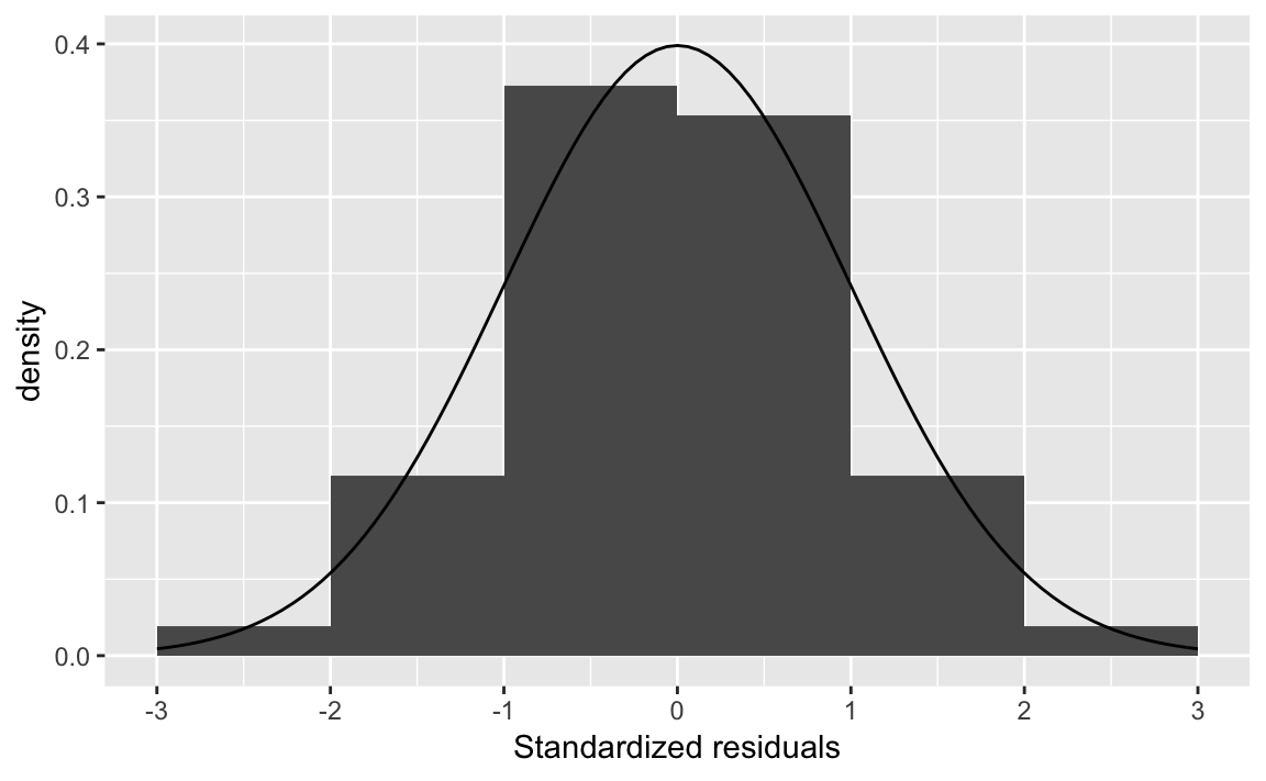

Obama’s vote shares in 2008 and 2012.

Standard deviation of errors:

err_sd <- sd(resid(fit1))

Probability of having a larger vote in California in 2012 than in 2008?

CA_2008 <- filter(pres, state == "CA")$Obama_2008_z

The predicted value of 2012 vote share can be calculated manually with \(\hat{beta} \times x\),

CA_mean_2012 <- CA_2008 * coef(fit1)["Obama_2008_z"]
CA_mean_2012
#> Obama_2008_z 
#>        0.858

or calculated using the predict function with the newdata argument providing any specific values to calculate?

predict(fit1, newdata = tibble(Obama_2008_z = CA_2008))
#>     1 
#> 0.858

Now calculate

pnorm(CA_2008, mean = CA_mean_2012, sd = err_sd,
      lower.tail = FALSE)
#> [1] 0.468

We can generalize the previous code to calculate the probability that Obama would exceed his 2008 vote to all states:

pres_gt_2008 <- augment(fit1) %>%
  mutate(p_greater = pnorm(Obama_2008_z, mean = .fitted, sd = err_sd,
                           lower.tail = FALSE))

Plotting these results, we can observe regression to the mean. States with larger (smaller) 2008 vote shares had a lower (higher) probability that the 2012 vote share will exceed them.

ggplot(pres_gt_2008, aes(x = Obama_2008_z, y = p_greater)) +
  modelr::geom_ref_line(h = 0.5) +
  modelr::geom_ref_line(v = 0) +
  geom_point() +
  labs(x = "Standardized vote share of Obama (2008)",
       y = "Pr. 2012 vote share greater than 2008")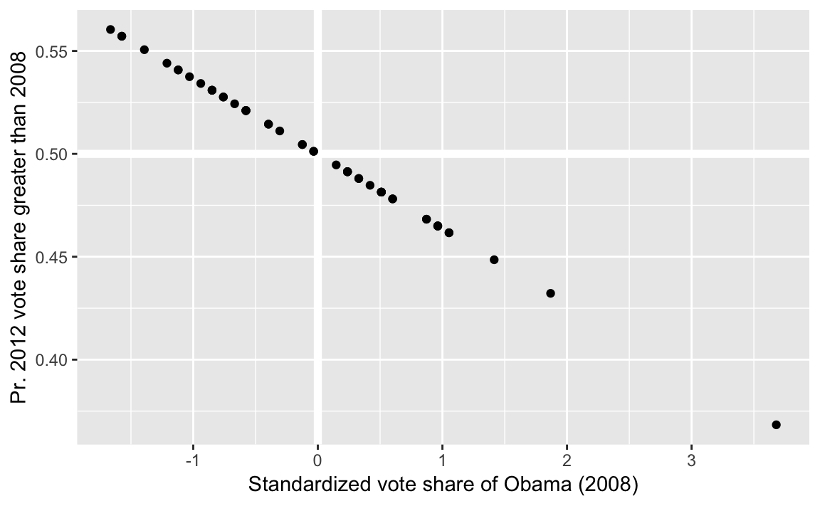

6.3.4 Expectation and Variance

Theoretical and actual sample variable of a set of Bernoulli draws:

p <- 0.5
# theretical variance
p * (1 - p)
#> [1] 0.25
# a sample
y <- sample(c(0, 1), size = 1000, replace = TRUE, prob = c(p, 1 - p))
# the sample variance of that sample
var(y)
#> [1] 0.25

6.3.5 Predicting Election Outcomes with Uncertainty

Load 2008 Presidential Election data:

data("pres08", package = "qss")
pres08 <- mutate(pres08, p = Obama / (Obama + McCain))

sim_election <- function(x, n = 1000) {
  n_states <- nrow(x)
  # samples the number of votes for Obama
  mutate(x,
         draws = rbinom(n_states, size = !!n, prob = p),
         obama_EV = EV * (draws > (!!n / 2))) %>%
    pluck("obama_EV") %>%
    sum()
}

This function returns the electoral votes for Obama for a single simulation:

sim_election(pres08)
#> [1] 353

Run this simulation sims times, saving the electoral votes of Obama in each simulation:

sims <- 10000
Obama_EV_sims <- map_dbl(seq_len(sims), ~ sim_election(pres08))

Obama’s actual electoral value

OBAMA_EV <- 364

library("glue")
ggplot(tibble(Obama_EV = Obama_EV_sims),
       aes(x = Obama_EV, y = ..density..)) +
  geom_histogram(binwidth = 10, boundary = 0, fill = "gray60") +
  geom_vline(xintercept = OBAMA_EV, colour = "black", size = 2) +
  annotate("text", x = OBAMA_EV + 2, y = 0.02,
           label = glue("Obama's 2008 EV = {OBAMA_EV}"), hjust = 0) +
  scale_x_continuous("Obama's Electoral College Votes",
                     breaks = seq(300, 400, by = 20)) +
  scale_y_continuous("Density") +
  labs(title = "Prediction of election outcomes")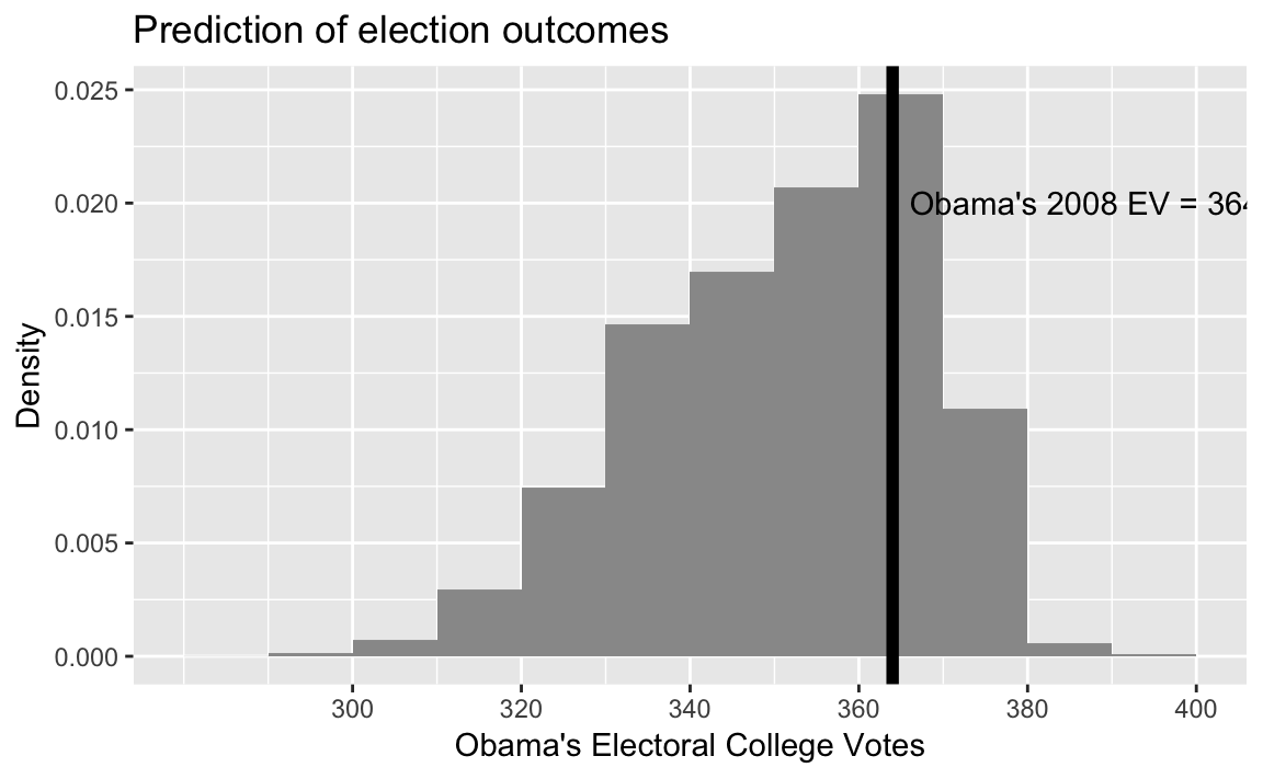

Summarize the simulations:

summary(Obama_EV_sims)
#>    Min. 1st Qu.  Median    Mean 3rd Qu.    Max. 
#>     289     340     353     352     364     398

Compare theoretical and simulation means:

# simulation EV
mean(Obama_EV_sims)
#> [1] 352
# theoretical
n <- 1000
pres08 %>%
  mutate(Obama_EV = EV * pbinom(n / 2, size = n, prob = p,
                                lower.tail = FALSE)) %>%
  summarise(Obama_EV = sum(Obama_EV))
#>   Obama_EV
#> 1      352

Compare theoretical and simulation variances:

# simulation variance
var(Obama_EV_sims)
#> [1] 269
# theoretical variance
Obama_EV_var <- pres08 %>%
  mutate(pb = pbinom(n / 2, size = n, prob = p, lower.tail = FALSE),
         EV_var = pb * (1 - pb) * EV ^ 2) %>%
  summarise(EV_var = sum(EV_var)) %>%
  pluck("EV_var")
Obama_EV_var
#> [1] 269

and standard deviations

# sim
sd(Obama_EV_sims)
#> [1] 16.4
# theoretical
sqrt(Obama_EV_var)
#> [1] 16.4

6.4 Large Sample Theorems

6.4.1 Law of Large Numbers

Put the simulation number, x and mean in a tibble:

sims <- 1000
p <- 0.2
size <- 10
lln_binom <- tibble(
  n = seq_len(sims),
  x = rbinom(sims, prob = p, size = size),
  mean = cumsum(x) / n,
  distrib = str_c("Binomial(", size, ", ", p, ")"))

lln_unif <-
 tibble(n = seq_len(sims),
        x = runif(sims),
        mean = cumsum(x) / n,
        distrib = str_c("Uniform(0, 1)"))

true_means <-
  tribble(~distrib, ~mean,
          "Uniform(0, 1)", 0.5,
          str_c("Binomial(", size, ", ", p, ")"), size * p)

ggplot() +
  geom_hline(aes(yintercept = mean), data = true_means,
             colour = "white", size = 2) +
  geom_line(aes(x = n, y = mean),
            data = bind_rows(lln_binom, lln_unif)) +
  facet_grid(distrib ~ ., scales = "free_y") +
  labs(x = "Sample Size", y = "Sample Mean")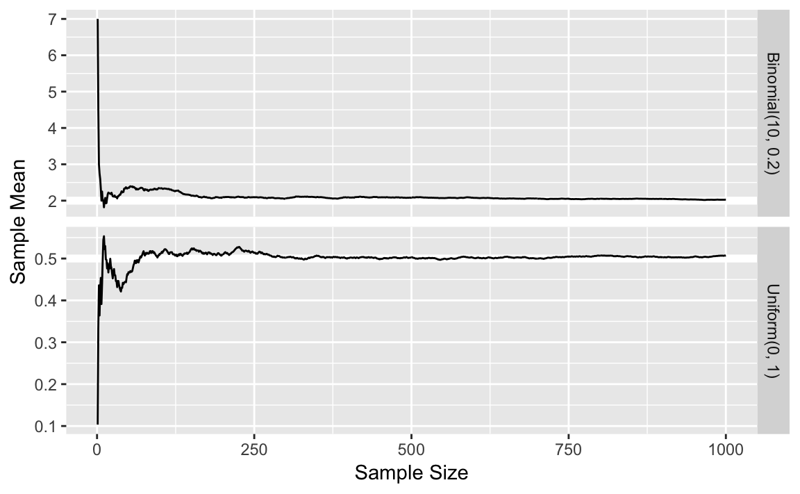

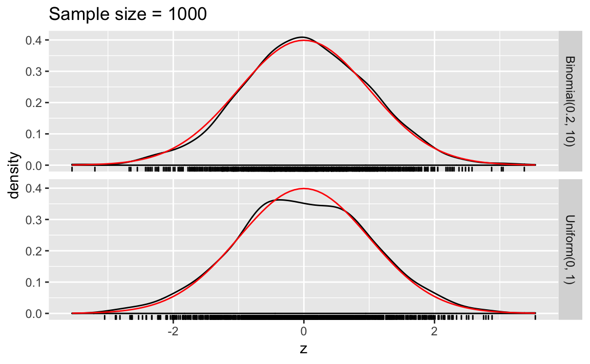
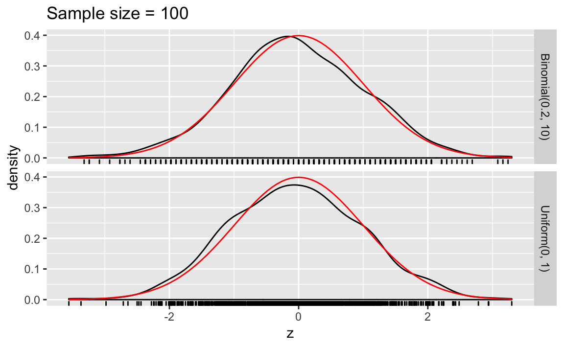
6.4.2 Central Limit Theorem

The population mean of the binomial distribution is \(\mu = p n\) and the variance is \(\sigma^2 = p (1 - p) n\).

sims <- 1000
n_samp <- 1000

Write functions to calculate the mean of a binomial distribution with size, size, and probability, p,

binom_mean <- function(size, p) {
  size * p
}

variance of a binomial distribution,

binom_var <- function(size, p) {
  size * p * (1 - p)
}

Write a function that takes n_samp samples from a binomial distribution with size, size, and probability of success, p, and returns a data frame with the z-score of the sample distribution:

sim_binom_clt <- function(n_samp, size, p) {
  x <- rbinom(n_samp, prob = p, size = size)
  z <- (mean(x) - binom_mean(size, p)) /
    sqrt(binom_var(size, p) / n_samp)
  tibble(distrib = str_c("Binomial(", p, ", ", size, ")"),
         z = z)
}

For the uniform distribution, we need a function to calculate the mean of a uniform distribution,

unif_mean <- function(min, max) {
  0.5 * (min + max)
}

variance of a uniform distribution,

unif_var <- function(min, max) {
  (1 / 12) * (max - min) ^ 2
}

and a function to perform the CLT simulation,

sim_unif_clt <- function(n_samp, min = 0, max = 1) {
  x <- runif(n_samp, min = min, max = max)
  z <- (mean(x) - unif_mean(min, max)) /
    sqrt(unif_var(min, max) / n_samp)
  tibble(distrib = str_c("Uniform(", min, ", ", max, ")"),
         z = z)
}

Since we will calculate this for n_samp = 1000 and n_samp, we might as well write a function for it.

clt_plot <- function(n_samp) {
  bind_rows(map_df(seq_len(sims), ~ sim_binom_clt(n_samp, size, p)),
            map_df(seq_len(sims), ~ sim_unif_clt(n_samp))) %>%
    ggplot(aes(x = z)) +
    geom_density() +
    geom_rug() +
    stat_function(fun = dnorm, colour = "red") +
    facet_grid(distrib ~ .) +
    ggtitle(str_c("Sample size = ", n_samp))
}
clt_plot(1000)
clt_plot(100)