7 Uncertainty
Prerequisites
We will use these package in this chapter:
library("tidyverse")
library("forcats")
library("lubridate")
library("stringr")
library("modelr")
library("broom")
library("purrr")
7.1 Estimation
7.1.1 Unbiasedness and Consistency
In these simulations, we draw a sample of size n from normal distributions with means mu0 and mu1 and standard deviations sd0 and sd1 respectively,
n <- 100
mu0 <- 0
sd0 <- 1
mu1 <- 1
sd1 <- 1
smpl <- tibble(id = seq_len(n),
               # Y if not treated
               Y0 = rnorm(n, mean = mu0, sd = sd0),
               # Y if treated
               Y1 = rnorm(n, mean = mu1, sd = sd1),
               # individual treatment effects
               tau = Y1 - Y0)
The SATE is:
SATE <- mean(smpl[["tau"]])
SATE
#> [1] 0.952
Simulations of RCTs. Write a function that takes the sample as an input smpl, then randomly assigns the treatment to each individual:
sim_treat <- function(smpl) {
  n <- nrow(smpl)
  SATE <- mean(smpl[["tau"]])
  # indexes of obs receiving treatment
  idx <- sample(seq_len(n), floor(nrow(smpl) / 2), replace = FALSE)
  # treat variable are those receiving treatment, else 0
  smpl[["treat"]] <- as.integer(seq_len(nrow(smpl)) %in% idx)
  smpl %>%
    mutate(Y_obs = if_else(treat == 1L, Y1, Y0)) %>%
    group_by(treat) %>%
    summarise(Y_obs = mean(Y_obs)) %>%
    spread(treat, Y_obs) %>%
    rename(Y1_mean = `1`, Y0_mean = `0`) %>%
    mutate(diff_mean = Y1_mean - Y0_mean,
           est_error = diff_mean - SATE)
}
This returns a data frame with columns: Y0_mean (mean \(Y\) for observations not receiving the treatment), Y1_mean (mean \(Y\) for observations receiving the treatment), diff (difference in mean values between the two groups), and est_error (difference between the estimated difference and the known SATE):
sim_treat(smpl)
#> # A tibble: 1 x 4
#>   Y0_mean Y1_mean diff_mean est_error
#>     <dbl>   <dbl>     <dbl>     <dbl>
#> 1 -0.0570   0.875     0.932   -0.0207
Rerun this function sims times:
sims <- 5000
sate_sims <- map_df(seq_len(sims), ~ sim_treat(smpl))
summary(sate_sims[["est_error"]])
#>    Min. 1st Qu.  Median    Mean 3rd Qu.    Max.
#>  -0.484  -0.087  -0.002  -0.001   0.085   0.414
Simulate the PATE:
PATE <- mu1 - mu0sim_pate <- function(n, mu0, mu1, sd0, sd1) {
smpl <- tibble(Y0 = rnorm(n, mean = mu0, sd = sd0),
Y1 = rnorm(n, mean = mu1, sd = sd1),
tau = Y1 - Y0)
# indexes of obs receiving treatment
idx <- sample(seq_len(n), floor(nrow(smpl) / 2), replace = FALSE)
# treat variable are those receiving treatment, else 0
smpl[["treat"]] <- as.integer(seq_len(nrow(smpl)) %in% idx)
smpl %>%
mutate(Y_obs = if_else(treat == 1L, Y1, Y0)) %>%
group_by(treat) %>%
summarise(Y_obs = mean(Y_obs)) %>%
spread(treat, Y_obs) %>%
rename(Y1_mean = `1`, Y0_mean = `0`) %>%
mutate(diff_mean = Y1_mean - Y0_mean,
est_error = diff_mean - PATE)
}Example of one simulation
sim_pate(n, mu0, mu1, sd0, sd1)
#> # A tibble: 1 x 4
#>   Y0_mean Y1_mean diff_mean est_error
#>     <dbl>   <dbl>     <dbl>     <dbl>
#> 1  -0.109   0.925      1.03    0.0338
pate_sims <-
map_df(seq_len(sims), ~ sim_pate(n, mu0, mu1, sd0, sd1))
summary(pate_sims[["est_error"]])
#> Min. 1st Qu. Median Mean 3rd Qu. Max.
#> -0.677 -0.135 -0.004 -0.003 0.129 0.8537.1.2 Standard Error
Plot of the sampling distribution of the difference-in-means estimator:
ggplot(pate_sims, aes(x = diff_mean, y = ..density..)) +
  geom_histogram(binwidth = 0.01, boundary = 1) +
  geom_vline(xintercept = PATE, colour = "white", size = 2) +
  ggtitle("Sampling distribution") +
  labs(x = "Difference-in-means estimator")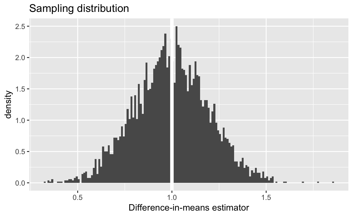
sd(pate_sims[["diff_mean"]])
#> [1] 0.196
Simulate PATE with a standard error:
sim_pate_se <- function(n, mu0, mu1, sd0, sd1) {
  # PATE - difference in means
  PATE <- mu1 - mu0
  # sample
  smpl <- tibble(Y0 = rnorm(n, mean = mu0, sd = sd0),
                 Y1 = rnorm(n, mean = mu1, sd = sd1),
                 tau = Y1 - Y0)
  # indexes of obs receiving treatment
  idx <- sample(seq_len(n), floor(nrow(smpl) / 2), replace = FALSE)
  # treat variable are those receiving treatment, else 0
  smpl[["treat"]] <- as.integer(seq_len(nrow(smpl)) %in% idx)
  # sample
  smpl %>%
    mutate(Y_obs = if_else(treat == 1L, Y1, Y0)) %>%
    group_by(treat) %>%
    summarise(mean = mean(Y_obs),
              var = var(Y_obs),
              nobs = n()) %>%
    summarise(diff_mean = diff(mean),
              se = sqrt(sum(var / nobs)),
              est_error = diff_mean - PATE)
}
Run a single simulation:
sim_pate_se(n, mu0, mu1, sd0, sd1)
#> # A tibble: 1 x 3
#>   diff_mean    se est_error
#>       <dbl> <dbl>     <dbl>
#> 1      1.05 0.190    0.0539
Run sims simulations:
sims <- 5000
pate_sims_se <-
  map_df(seq_len(sims), ~ sim_pate_se(n, mu0, mu1, sd0, sd1))
Standard deviation of difference-in-means
sd(pate_sims_se[["diff_mean"]])
#> [1] 0.199
Mean of standard errors,
mean(pate_sims_se[["se"]])
#> [1] 0.2
7.1.3 Confidence Intervals
Calculate a \(p\%\) confidence interval for the binomial distribution:
# Sample size
n <- 1000
# point estimate
x_bar <- 0.6
# standard error
se <- sqrt(x_bar * (1 - x_bar) / n)
# Desired Confidence levels
levels <- c(0.99, 0.95, 0.90)tibble(level = levels) %>%
mutate(
ci_lower = x_bar - qnorm(1 - (1 - level) / 2) * se,
ci_upper = x_bar + qnorm(1 - (1 - level) / 2) * se
)
#> # A tibble: 3 x 3
#> level ci_lower ci_upper
#> <dbl> <dbl> <dbl>
#> 1 0.99 0.560 0.640
#> 2 0.95 0.570 0.630
#> 3 0.9 0.575 0.625Calculate the coverage ratio of the 95% confidence interval in the PATE simulations.
level <- 0.95
pate_sims_se %>%
  mutate(ci_lower = diff_mean - qnorm(1 - (1 - level) / 2) * se,
         ci_upper = diff_mean + qnorm(1 - (1 - level) / 2) * se,
         includes_pate = PATE > ci_lower & PATE < ci_upper) %>%
  summarise(coverage = mean(includes_pate))
#> # A tibble: 1 x 1
#>   coverage
#>      <dbl>
#> 1    0.948
To do this for multiple levels encapsulate the above code in a function with arguments .data (the data frame) and the confidence level, level:
pate_sims_coverage <- function(.data, level = 0.95) {
  mutate(.data,
         ci_lower = diff_mean - qnorm(1 - (1 - level) / 2) * se,
         ci_upper = diff_mean + qnorm(1 - (1 - level) / 2) * se,
         includes_pate = PATE > ci_lower & PATE < ci_upper) %>%
    summarise(coverage = mean(includes_pate))
}

pate_sims_coverage(pate_sims_se, 0.95)
#> # A tibble: 1 x 1
#>   coverage
#>      <dbl>
#> 1    0.948
pate_sims_coverage(pate_sims_se, 0.99)
#> # A tibble: 1 x 1
#>   coverage
#>      <dbl>
#> 1    0.989
pate_sims_coverage(pate_sims_se, 0.90)
#> # A tibble: 1 x 1
#>   coverage
#>      <dbl>
#> 1    0.898
p <- 0.6
n <- 10
alpha <- 0.05
sims <- 5000Define a function that samples from a Bernoulli distribution, calculates its standard error, and returns a logical value as to whether it contains the true value:
binom_ci_contains <- function(n, p, alpha = 0.05) {
  x <- rbinom(n, size = 1, prob = p)
  x_bar <- mean(x)
  se <- sqrt(x_bar * (1 - x_bar) / n)
  ci_lower <- x_bar - qnorm(1 - alpha / 2) * se
  ci_upper <- x_bar + qnorm(1 - alpha / 2) * se
  (ci_lower <= p) & (p <= ci_upper)
}
We can run this once for given sample size:
n <- 10
binom_ci_contains(n, p)
#> [1] FALSE
Using map_df we can rerun it sims times and calculate the coverage proportion:
mean(map_lgl(seq_len(sims), ~ binom_ci_contains(n, p)))
#> [1] 0.905
Encapsulate the above code in a function that calculates the coverage of a confidence interval with size, n, and success probability, p:
binom_ci_coverage <- function(n, p, sims) {
  mean(map_lgl(seq_len(sims), ~ binom_ci_contains(n, p)))
}
Use binom_ci_coverage to calculate CI coverage for multiple values of the sample size:
tibble(n = c(10L, 100L, 1000L)) %>%
  mutate(coverage = map_dbl(n, binom_ci_coverage, p = !!p, sims = !!sims))
#> # A tibble: 3 x 2
#>       n coverage
#>   <int>    <dbl>
#> 1    10    0.900
#> 2   100    0.943
#> 3  1000    0.948
7.1.4 Margin of Error and Sample Size Calculation in Polls
Write a function to calculate the sample size needed for a given proportion.
moe_pop_prop <- function(MoE) {
  tibble(p = seq(from = 0.01, to = 0.99, by = 0.01),
         n = 1.96 ^ 2 * p * (1 - p) / MoE ^ 2,
         MoE = MoE)
}
moe_pop_prop(0.01)
#> # A tibble: 99 x 3
#>       p     n   MoE
#>   <dbl> <dbl> <dbl>
#> 1  0.01  380.  0.01
#> 2  0.02  753.  0.01
#> 3  0.03 1118.  0.01
#> 4  0.04 1475.  0.01
#> 5  0.05 1825.  0.01
#> 6  0.06 2167.  0.01
#> # ... with 93 more rows
Then use map_df to call this function for different margins of error, and return the entire thing as a data frame with columns: n, p, and MoE.
MoE <- c(0.01, 0.03, 0.05)
props <- map_df(MoE, moe_pop_prop)
Since its a data frame, its easy to plot with ggplot:
ggplot(props, aes(x = p, y = n, colour = factor(MoE))) +
geom_line() +
labs(colour = "margin of error",
x = "population proportion",
y = "sample size") +
theme(legend.position = "bottom")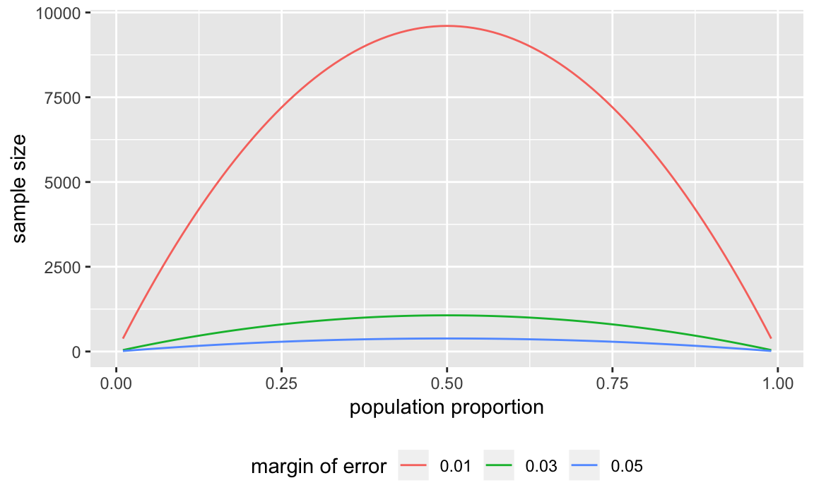 read_csv already recognizes the date columns, so we don’t need to convert them. The 2008 election was on Nov 11, 2008, so we’ll store that in a variable.
ELECTION_DATE <- ymd(20081104)Load the final vote shares,
data("pres08", package = "qss")and polling data
data("polls08", package = "qss")We need to add an additional column to the polls08 data frame which contains the number of days until the election:
polls08 <- polls08 %>%
  mutate(DaysToElection = as.integer(ELECTION_DATE - middate))
For each state calculate the mean of the latest polls,
poll_pred <-
  polls08 %>%
  group_by(state) %>%
  # latest polls in the state
  filter(DaysToElection == min(DaysToElection)) %>%
  # take mean of latest polls and convert from 0-100 to 0-1
  summarise(Obama = mean(Obama) / 100)
# Add confidence itervals
# sample size
sample_size <- 1000
# confidence level
alpha <- 0.05
poll_pred <-
  poll_pred %>%
  mutate(se = sqrt(Obama * (1 - Obama) / sample_size),
         ci_lwr = Obama + qnorm(alpha / 2) * se,
         ci_upr = Obama + qnorm(1 - alpha / 2) * se)
# Add actual outcome
poll_pred <-
  left_join(poll_pred,
            select(pres08, state, actual = Obama),
            by = "state") %>%
  mutate(actual = actual / 100,
         covers = (ci_lwr <= actual) & (actual <= ci_upr))
poll_pred
#> # A tibble: 51 x 7
#>   state Obama     se ci_lwr ci_upr actual covers
#>   <chr> <dbl>  <dbl>  <dbl>  <dbl>  <dbl> <lgl>
#> 1 AK    0.39  0.0154  0.360  0.420   0.38 TRUE
#> 2 AL    0.36  0.0152  0.330  0.390   0.39 FALSE
#> 3 AR    0.44  0.0157  0.409  0.471   0.39 FALSE
#> 4 AZ    0.465 0.0158  0.434  0.496   0.45 TRUE
#> 5 CA    0.6   0.0155  0.570  0.630   0.61 TRUE
#> 6 CO    0.52  0.0158  0.489  0.551   0.54 TRUE
#> # ... with 45 more rows
In the plot, color the point ranges by whether they include the election day outcome.
ggplot(poll_pred, aes(x = actual, y = Obama,
                      ymin = ci_lwr, ymax = ci_upr,
                      colour = covers)) +
  geom_abline(intercept = 0, slope = 1, colour = "white", size = 2) +
  geom_pointrange() +
  scale_y_continuous("Poll prediction", limits = c(0, 1)) +
  scale_x_continuous("Obama's vote share", limits = c(0, 1)) +
  scale_colour_discrete("CI includes result?") +
  coord_fixed() +
  theme(legend.position = "bottom")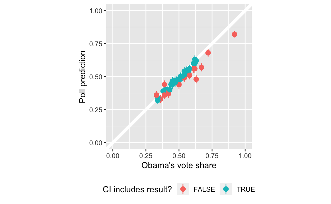
Proportion of polls with confidence intervals that include the election outcome?
poll_pred %>%
  summarise(mean(covers))
#> # A tibble: 1 x 1
#>   `mean(covers)`
#>            <dbl>
#> 1          0.588
poll_pred <-
poll_pred %>%
# calc bias
mutate(bias = Obama - actual) %>%
# bias corrected prediction, se, and CI
mutate(Obama_bc = Obama - mean(bias),
se_bc = sqrt(Obama_bc * (1 - Obama_bc) / sample_size),
ci_lwr_bc = Obama_bc + qnorm(alpha / 2) * se_bc,
ci_upr_bc = Obama_bc + qnorm(1 - alpha / 2) * se_bc,
covers_bc = (ci_lwr_bc <= actual) & (actual <= ci_upr_bc))
poll_pred %>%
summarise(mean(covers_bc))
#> # A tibble: 1 x 1
#> `mean(covers_bc)`
#> <dbl>
#> 1 0.7657.1.5 Analysis of Randomized Controlled Trials
Load the STAR data from the qss package,
data("STAR", package = "qss")Add meaningful labels to the classtype variable:
STAR <- STAR %>%
  mutate(classtype = factor(classtype,
                            labels = c("small class", "regular class",
                                       "regular class with aid")))
Summarize scores by classroom type:
classtype_means <-
  STAR %>%
  group_by(classtype) %>%
  summarise(g4reading = mean(g4reading, na.rm = TRUE))
Plot the distribution of scores by classroom type:
classtypes_used <- c("small class", "regular class")
ggplot(filter(STAR,
              classtype %in% classtypes_used,
              !is.na(g4reading)),
       aes(x = g4reading, y = ..density..)) +
  geom_histogram(binwidth = 20) +
  geom_vline(data = filter(classtype_means, classtype %in% classtypes_used),
             mapping = aes(xintercept = g4reading),
             colour = "white", size = 2) +
  facet_grid(classtype ~ .) +
  labs(x = "Fourth grade reading score", y = "Density")

alpha <- 0.05
star_estimates <-
  STAR %>%
  filter(!is.na(g4reading)) %>%
  group_by(classtype) %>%
  summarise(n = n(),
            est = mean(g4reading),
            se = sd(g4reading) / sqrt(n)) %>%
  mutate(lwr = est + qnorm(alpha / 2) * se,
         upr = est + qnorm(1 - alpha / 2) * se)
star_estimates
#> # A tibble: 3 x 6
#>   classtype                  n   est    se   lwr   upr
#>   <fct>                  <int> <dbl> <dbl> <dbl> <dbl>
#> 1 small class              726  723.  1.91  720.  727.
#> 2 regular class            836  720.  1.84  716.  723.
#> 3 regular class with aid   791  721.  1.86  717.  724.

star_estimates %>%
  filter(classtype %in% c("small class", "regular class")) %>%
  # ensure that it is ordered small then regular
  arrange(desc(classtype)) %>%
  summarise(
    se = sqrt(sum(se ^ 2)),
    est = diff(est)
  ) %>%
  mutate(ci_lwr = est + qnorm(alpha / 2) * se,
         ci_up = est + qnorm(1 - alpha / 2) * se)
#> # A tibble: 1 x 4
#>      se   est ci_lwr ci_up
#>   <dbl> <dbl>  <dbl> <dbl>
#> 1  2.65  3.50  -1.70  8.70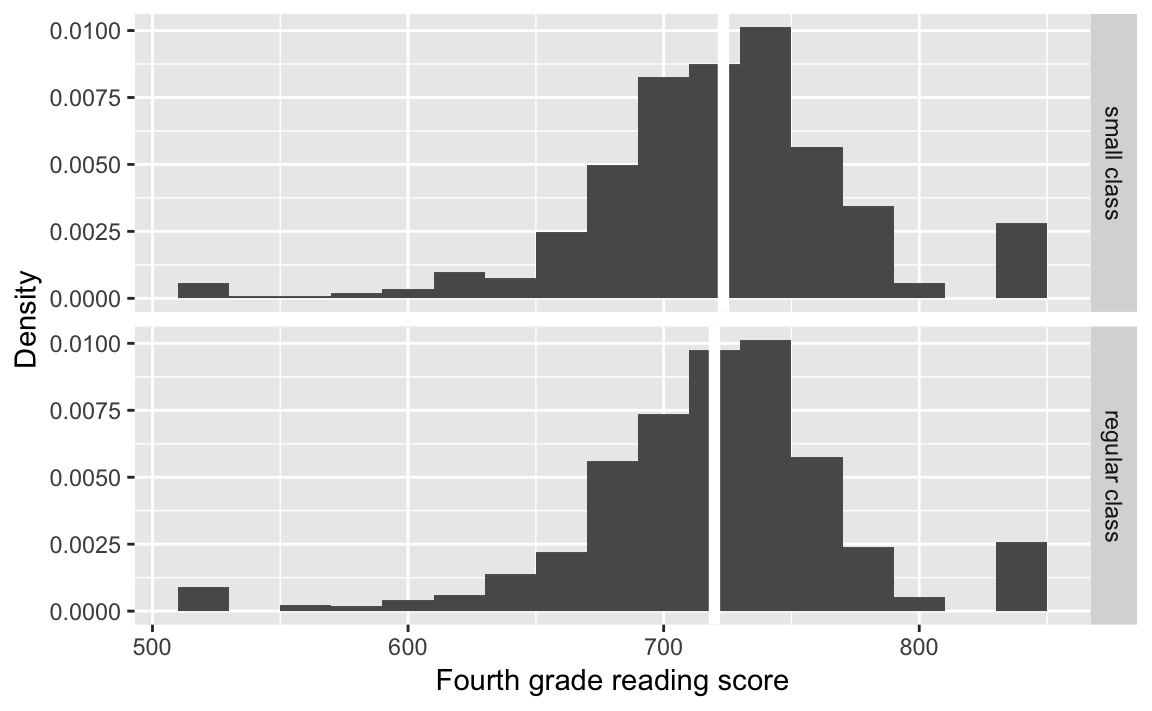
Use we could use spread and gather:
star_ate <-
  star_estimates %>%
  filter(classtype %in% c("small class", "regular class")) %>%
  mutate(classtype = fct_recode(factor(classtype),
                                "small" = "small class",
                                "regular" = "regular class")) %>%
  select(classtype, est, se) %>%
  gather(stat, value, -classtype) %>%
  unite(variable, stat, classtype)  %>%
  spread(variable, value) %>%
  mutate(ate_est = est_small - est_regular,
         ate_se = sqrt(se_small ^ 2 + se_regular ^ 2),
         ci_lwr = ate_est + qnorm(alpha / 2) * ate_se,
         ci_upr = ate_est + qnorm(1 - alpha / 2) * ate_se)
star_ate
#> # A tibble: 1 x 8
#>   est_regular est_small se_regular se_small ate_est ate_se ci_lwr ci_upr
#>         <dbl>     <dbl>      <dbl>    <dbl>   <dbl>  <dbl>  <dbl>  <dbl>
#> 1        720.      723.       1.84     1.91    3.50   2.65  -1.70   8.70
7.1.6 Analysis Based on Student’s t-Distribution
Use filter to subset.
t.test(filter(STAR, classtype == "small class")$g4reading,
       filter(STAR, classtype == "regular class")$g4reading)
#>
#>  Welch Two Sample t-test
#>
#> data:  filter(STAR, classtype == "small class")$g4reading and filter(STAR, classtype == "regular class")$g4reading
#> t = 1, df = 2000, p-value = 0.2
#> alternative hypothesis: true difference in means is not equal to 0
#> 95 percent confidence interval:
#>  -1.70  8.71
#> sample estimates:
#> mean of x mean of y
#>       723       720
The function t.test can also take a formula as its first parameter.
t.test(g4reading ~ classtype,
       data = filter(STAR, classtype %in% c("small class", "regular class")))
#>
#>  Welch Two Sample t-test
#>
#> data:  g4reading by classtype
#> t = 1, df = 2000, p-value = 0.2
#> alternative hypothesis: true difference in means is not equal to 0
#> 95 percent confidence interval:
#>  -1.70  8.71
#> sample estimates:
#>   mean in group small class mean in group regular class
#>                         723                         720
7.2 Hypothesis Testing
7.2.1 Tea-Testing Experiment
# Number of cups of tea
cups <- 4
# Number guessed correctly
k <- c(0, seq_len(cups))
true <-  tibble(correct = k * 2,
                n = choose(cups, k) * choose(cups, cups - k)) %>%
  mutate(prob = n / sum(n))
true
#> # A tibble: 5 x 3
#>   correct     n   prob
#>     <dbl> <dbl>  <dbl>
#> 1       0     1 0.0143
#> 2       2    16 0.229
#> 3       4    36 0.514
#> 4       6    16 0.229
#> 5       8     1 0.0143

sims <- 1000
guess <- tibble(guess = c("M", "T", "T", "M", "M", "T", "T", "M"))
randomize_tea <- function(df) {
  # randomize the order of teas
  assignment <- sample_frac(df, 1) %>%
    rename(actual = guess)
  bind_cols(df, assignment) %>%
    summarise(correct = sum(guess == actual))
}
approx <-
  map_df(seq_len(sims), ~ randomize_tea(guess)) %>%
  count(correct) %>%
  mutate(prob = n / sum(n))
left_join(select(approx, correct, prob_sim = prob),
          select(true, correct, prob_exact = prob),
          by = "correct") %>%
  mutate(diff = prob_sim - prob_exact)
#> # A tibble: 5 x 4
#>   correct prob_sim prob_exact     diff
#>     <dbl>    <dbl>      <dbl>    <dbl>
#> 1       0    0.011     0.0143 -0.00329
#> 2       2    0.234     0.229   0.00543
#> 3       4    0.486     0.514  -0.0283
#> 4       6    0.253     0.229   0.0244
#> 5       8    0.016     0.0143  0.00171
7.2.2 The General Framework
The test functions like fisher.test do not work particularly well with data frames, and expect vectors or matrices as input, so tidyverse functions are less directly applicable
# all guesses correct
x <- tribble(~Guess, ~Truth, ~Number,
             "Milk", "Milk", 4L,
             "Milk", "Tea", 0L,
             "Tea", "Milk", 0L,
             "Tea", "Tea", 4L)
x
#> # A tibble: 4 x 3
#>   Guess Truth Number
#>   <chr> <chr>  <int>
#> 1 Milk  Milk       4
#> 2 Milk  Tea        0
#> 3 Tea   Milk       0
#> 4 Tea   Tea        4
# 6 correct guesses
y <- x %>%
  mutate(Number = c(3L, 1L, 1L, 3L))
y
#> # A tibble: 4 x 3
#>   Guess Truth Number
#>   <chr> <chr>  <int>
#> 1 Milk  Milk       3
#> 2 Milk  Tea        1
#> 3 Tea   Milk       1
#> 4 Tea   Tea        3
# Turn into a 2x2 table for fisher.test
select(spread(x, Truth, Number), -Guess)
#> # A tibble: 2 x 2
#>    Milk   Tea
#>   <int> <int>
#> 1     4     0
#> 2     0     4
# Use spread to make it a 2 x 2 table
fisher.test(select(spread(x, Truth, Number), -Guess),
            alternative = "greater")
#>
#>  Fisher's Exact Test for Count Data
#>
#> data:  select(spread(x, Truth, Number), -Guess)
#> p-value = 0.01
#> alternative hypothesis: true odds ratio is greater than 1
#> 95 percent confidence interval:
#>    2 Inf
#> sample estimates:
#> odds ratio
#>        Inf
fisher.test(select(spread(y, Truth, Number), -Guess))
#>
#>  Fisher's Exact Test for Count Data
#>
#> data:  select(spread(y, Truth, Number), -Guess)
#> p-value = 0.5
#> alternative hypothesis: true odds ratio is not equal to 1
#> 95 percent confidence interval:
#>    0.212 621.934
#> sample estimates:
#> odds ratio
#>       6.41
7.2.3 One-Sample Tests
n <- 1018
x_bar <- 550 / n
se <- sqrt(0.5 * 0.5 / n) # standard deviation of sampling distribution
# upper red area in the figure
upper <- pnorm(x_bar, mean = 0.5, sd = se, lower.tail = FALSE)
# lower red area in the figure; identical to the upper area
lower <- pnorm(0.5 - (x_bar - 0.5), mean = 0.5, sd = se)
# two side p value
upper + lower
#> [1] 0.0102
2 * upper
#> [1] 0.0102
# one sided p value
upper
#> [1] 0.00508
z_score <- (x_bar - 0.5) / se
z_score
#> [1] 2.57
pnorm(z_score, lower.tail = FALSE) # one-sided p-value
#> [1] 0.00508
2 * pnorm(z_score, lower.tail = FALSE) # two-sided p-value
#> [1] 0.0102
# 99% confidence interval contains 0.5
c(x_bar - qnorm(0.995) * se, x_bar + qnorm(0.995) * se)
#> [1] 0.500 0.581
# 95% confidence interval does not contain 0.5
c(x_bar - qnorm(0.975) * se, x_bar + qnorm(0.975) * se)
#> [1] 0.510 0.571
# no continuity correction to get the same p-value as above
prop.test(550, n = n, p = 0.5, correct = FALSE)
#>
#>  1-sample proportions test without continuity correction
#>
#> data:  550 out of n, null probability 0.5
#> X-squared = 7, df = 1, p-value = 0.01
#> alternative hypothesis: true p is not equal to 0.5
#> 95 percent confidence interval:
#>  0.510 0.571
#> sample estimates:
#>    p
#> 0.54
# with continuity correction
prop.test(550, n = n, p = 0.5)
#>
#>  1-sample proportions test with continuity correction
#>
#> data:  550 out of n, null probability 0.5
#> X-squared = 6, df = 1, p-value = 0.01
#> alternative hypothesis: true p is not equal to 0.5
#> 95 percent confidence interval:
#>  0.509 0.571
#> sample estimates:
#>    p
#> 0.54
prop.test(550, n = n, p = 0.5, conf.level = 0.99)
#>
#>  1-sample proportions test with continuity correction
#>
#> data:  550 out of n, null probability 0.5
#> X-squared = 6, df = 1, p-value = 0.01
#> alternative hypothesis: true p is not equal to 0.5
#> 99 percent confidence interval:
#>  0.499 0.581
#> sample estimates:
#>    p
#> 0.54
# two-sided one-sample t-test
t.test(STAR$g4reading, mu = 710)
#>
#> One Sample t-test
#>
#> data: STAR$g4reading
#> t = 10, df = 2000, p-value <2e-16
#> alternative hypothesis: true mean is not equal to 710
#> 95 percent confidence interval:
#> 719 723
#> sample estimates:
#> mean of x
#> 7217.2.4 Two-sample tests
The ATE estimates are stored in a data frame, star_ate. Note that the dplyr function transmute is like mutate, but only returns the variables specified in the function.
star_ate %>%
  transmute(p_value_1sided = pnorm(-abs(ate_est),
                                   mean = 0, sd = ate_se),
            p_value_2sided = 2 * pnorm(-abs(ate_est), mean = 0,
                                   sd = ate_se))
#> # A tibble: 1 x 2
#>   p_value_1sided p_value_2sided
#>            <dbl>          <dbl>
#> 1         0.0935          0.187

t.test(g4reading ~ classtype,
  data = filter(STAR, classtype %in% c("small class", "regular class")))
#>
#>  Welch Two Sample t-test
#>
#> data:  g4reading by classtype
#> t = 1, df = 2000, p-value = 0.2
#> alternative hypothesis: true difference in means is not equal to 0
#> 95 percent confidence interval:
#>  -1.70  8.71
#> sample estimates:
#>   mean in group small class mean in group regular class
#>                         723                         720
or
t.test(filter(STAR, classtype == "small class")$g4reading,
       filter(STAR, classtype == "regular class")$g4reading)
#>
#>  Welch Two Sample t-test
#>
#> data:  filter(STAR, classtype == "small class")$g4reading and filter(STAR, classtype == "regular class")$g4reading
#> t = 1, df = 2000, p-value = 0.2
#> alternative hypothesis: true difference in means is not equal to 0
#> 95 percent confidence interval:
#>  -1.70  8.71
#> sample estimates:
#> mean of x mean of y
#> 723 720data("resume", package = "qss")
x <- resume %>%
count(race, call) %>%
spread(call, n) %>%
ungroup()
x
#> # A tibble: 2 x 3
#> race `0` `1`
#> <chr> <int> <int>
#> 1 black 2278 157
#> 2 white 2200 235
prop.test(as.matrix(select(x, -race)), alternative = "greater")
#>
#> 2-sample test for equality of proportions with continuity
#> correction
#>
#> data: as.matrix(select(x, -race))
#> X-squared = 20, df = 1, p-value = 2e-05
#> alternative hypothesis: greater
#> 95 percent confidence interval:
#> 0.0188 1.0000
#> sample estimates:
#> prop 1 prop 2
#> 0.936 0.903Assign sample sizes and proportions, then calculate point estimates, standard error, z-statistic and one-sided p-value.
n0 <- sum(resume$race == "black")
n1 <- sum(resume$race == "white")

p <- mean(resume$call)
p0 <- mean(filter(resume, race == "black")$call)
p1 <- mean(filter(resume, race == "white")$call)

est <- p1 - p0
est
#> [1] 0.032

se <- sqrt(p * (1 - p) * (1 / n0 + 1 / n1))
se
#> [1] 0.0078

zstat <- est / se
zstat
#> [1] 4.11

pnorm(-abs(zstat))
#> [1] 1.99e-05
The only thing that changed is using filter for selecting the groups.
7.2.5 Power Analysis
Set the parameters: the sample size,
n <- 250the population proportional under the alternative data generating process,
p_star <- 0.48the null hypothesis,
p <- 0.5the p-value,
alpha <- 0.05and
cr_value <- qnorm(1 - alpha / 2)The standard errors under the hypothetical data generating process is
se_star <- sqrt(p_star * (1 - p_star) / n)and the standard error under the null is
se <- sqrt(p * (1 - p) / n)The power for this test is
pnorm(p - cr_value * se, mean = p_star, sd = se_star) +
    pnorm(p + cr_value * se, mean = p_star, sd = se_star,
          lower.tail = FALSE)
#> [1] 0.0967
The parameters (sample sizes and proportions) are
n1 <- 500
n0 <- 500
p1_star <- 0.05
p0_star <- 0.1
Calculate the overall call back rate as a weighted average,
p <- (n1 * p1_star + n0 * p0_star) / (n1 + n0)the standard error under the null,
se <- sqrt(p * (1 - p) * (1 / n1 + 1 / n0))the standard error under the hypothetical data generating process,
se.star <- sqrt(p1_star * (1 - p1_star) / n1 + p0_star * (1 - p0_star) / n0)pnorm(-cr_value * se, mean = p1_star - p0_star, sd = se.star) +
pnorm(cr_value * se, mean = p1_star - p0_star, sd = se.star,
lower.tail = FALSE)
#> [1] 0.852power.prop.test(n = 500, p1 = 0.05, p2 = 0.1, sig.level = 0.05)
#>
#> Two-sample comparison of proportions power calculation
#>
#> n = 500
#> p1 = 0.05
#> p2 = 0.1
#> sig.level = 0.05
#> power = 0.852
#> alternative = two.sided
#>
#> NOTE: n is number in *each* grouppower.prop.test(p1 = 0.05, p2 = 0.1, sig.level = 0.05, power = 0.9)
#>
#> Two-sample comparison of proportions power calculation
#>
#> n = 581
#> p1 = 0.05
#> p2 = 0.1
#> sig.level = 0.05
#> power = 0.9
#> alternative = two.sided
#>
#> NOTE: n is number in *each* grouppower.t.test(n = 100, delta = 0.25, sd = 1, type = "one.sample")
#>
#> One-sample t test power calculation
#>
#> n = 100
#> delta = 0.25
#> sd = 1
#> sig.level = 0.05
#> power = 0.697
#> alternative = two.sidedpower.t.test(power = 0.9, delta = 0.25, sd = 1, type = "one.sample")
#>
#> One-sample t test power calculation
#>
#> n = 170
#> delta = 0.25
#> sd = 1
#> sig.level = 0.05
#> power = 0.9
#> alternative = two.sidedpower.t.test(delta = 0.25, sd = 1, type = "two.sample",
alternative = "one.sided", power = 0.9)
#>
#> Two-sample t test power calculation
#>
#> n = 275
#> delta = 0.25
#> sd = 1
#> sig.level = 0.05
#> power = 0.9
#> alternative = one.sided
#>
#> NOTE: n is number in *each* group7.3 Linear Regression Model with Uncertainty
7.3.1 Linear Regression as a Generative Model
Load the minimum wage date included with the qss package:
data("minwage", package = "qss")minwage <- mutate(minwage,
fullPropBefore = fullBefore / (fullBefore + partBefore),
fullPropAfter = fullAfter / (fullAfter + partAfter),
NJ = as.integer(location == "PA"))fit_minwage <- lm(fullPropAfter ~ -1 + NJ + fullPropBefore +
wageBefore + chain, data = minwage)
fit_minwage
#>
#> Call:
#> lm(formula = fullPropAfter ~ -1 + NJ + fullPropBefore + wageBefore +
#> chain, data = minwage)
#>
#> Coefficients:
#> NJ fullPropBefore wageBefore chainburgerking
#> -0.0542 0.1688 0.0813 -0.0614
#> chainkfc chainroys chainwendys
#> -0.0966 -0.1522 -0.1659
fit_minwage1 <- lm(fullPropAfter ~ NJ + fullPropBefore +
wageBefore + chain, data = minwage)
fit_minwage1
#>
#> Call:
#> lm(formula = fullPropAfter ~ NJ + fullPropBefore + wageBefore +
#> chain, data = minwage)
#>
#> Coefficients:
#> (Intercept) NJ fullPropBefore wageBefore
#> -0.0614 -0.0542 0.1688 0.0813
#> chainkfc chainroys chainwendys
#> -0.0352 -0.0908 -0.1045
gather_predictions(slice(minwage, 1), fit_minwage, fit_minwage1) %>%
select(model, pred)
#> model pred
#> 1 fit_minwage 0.271
#> 2 fit_minwage1 0.2717.3.2 Inference about coefficients
Use the tidy function to return the coefficients, including confidence intervals, as a data frame:
data("women", package = "qss")
fit_women <- lm(water ~ reserved, data = women)
summary(fit_women)
#>
#> Call:
#> lm(formula = water ~ reserved, data = women)
#>
#> Residuals:
#>    Min     1Q Median     3Q    Max
#> -23.99 -14.74  -7.86   2.26 316.01
#>
#> Coefficients:
#>             Estimate Std. Error t value Pr(>|t|)
#> (Intercept)    14.74       2.29    6.45  4.2e-10 ***
#> reserved        9.25       3.95    2.34     0.02 *
#> ---
#> Signif. codes:  0 '***' 0.001 '**' 0.01 '*' 0.05 '.' 0.1 ' ' 1
#>
#> Residual standard error: 33.4 on 320 degrees of freedom
#> Multiple R-squared:  0.0169, Adjusted R-squared:  0.0138
#> F-statistic: 5.49 on 1 and 320 DF,  p-value: 0.0197
tidy(fit_women)
#>          term estimate std.error statistic  p.value
#> 1 (Intercept)    14.74      2.29      6.45 4.22e-10
#> 2    reserved     9.25      3.95      2.34 1.97e-02
You need to set conf.int = TRUE for tidy to include the confidence interval:
summary(fit_minwage)
#>
#> Call:
#> lm(formula = fullPropAfter ~ -1 + NJ + fullPropBefore + wageBefore +
#>     chain, data = minwage)
#>
#> Residuals:
#>     Min      1Q  Median      3Q     Max
#> -0.4862 -0.1813 -0.0281  0.1513  0.7509
#>
#> Coefficients:
#>                 Estimate Std. Error t value Pr(>|t|)
#> NJ               -0.0542     0.0332   -1.63   0.1034
#> fullPropBefore    0.1688     0.0566    2.98   0.0031 **
#> wageBefore        0.0813     0.0389    2.09   0.0374 *
#> chainburgerking  -0.0614     0.1755   -0.35   0.7266
#> chainkfc         -0.0966     0.1793   -0.54   0.5904
#> chainroys        -0.1522     0.1832   -0.83   0.4066
#> chainwendys      -0.1659     0.1853   -0.90   0.3711
#> ---
#> Signif. codes:  0 '***' 0.001 '**' 0.01 '*' 0.05 '.' 0.1 ' ' 1
#>
#> Residual standard error: 0.244 on 351 degrees of freedom
#> Multiple R-squared:  0.635,  Adjusted R-squared:  0.628
#> F-statistic: 87.2 on 7 and 351 DF,  p-value: <2e-16
tidy(fit_minwage, conf.int = TRUE)
#>              term estimate std.error statistic p.value conf.low conf.high
#> 1              NJ  -0.0542    0.0332    -1.633 0.10343 -0.11953    0.0111
#> 2  fullPropBefore   0.1688    0.0566     2.981 0.00307  0.05744    0.2801
#> 3      wageBefore   0.0813    0.0389     2.090 0.03737  0.00478    0.1579
#> 4 chainburgerking  -0.0614    0.1755    -0.350 0.72657 -0.40648    0.2837
#> 5        chainkfc  -0.0966    0.1793    -0.539 0.59044 -0.44919    0.2560
#> 6       chainroys  -0.1522    0.1832    -0.831 0.40664 -0.51238    0.2080
#> 7     chainwendys  -0.1659    0.1853    -0.895 0.37115 -0.53031    0.1985
7.3.3 Inference about predictions
data("MPs", package = "qss")
MPs_labour <- filter(MPs, party == "labour")
MPs_tory <- filter(MPs, party == "tory")
labour_fit1 <- lm(ln.net ~ margin, data = filter(MPs_labour, margin < 0))
labour_fit2 <- lm(ln.net ~ margin, data = filter(MPs_labour, margin > 0))
tory_fit1 <- lm(ln.net ~ margin, data = filter(MPs_tory, margin < 0))
tory_fit2 <- lm(ln.net ~ margin, data = filter(MPs_tory, margin > 0))
Predictions at the threshold. The broom function augment will return prediction fitted values and standard errors for each value, but not the confidence intervals themselves (we’d have to multiply the correct t-distribution with degrees of freedom.) So instead, we’ll directly use the predict function:
tory_y0 <-
  predict(tory_fit1, interval = "confidence",
          newdata = tibble(margin = 0)) %>% as_tibble()
tory_y0
#> # A tibble: 1 x 3
#>     fit   lwr   upr
#>   <dbl> <dbl> <dbl>
#> 1  12.5  12.1  13.0
tory_y1 <-
  predict(tory_fit2, interval = "confidence",
          newdata = tibble(margin = 0)) %>% as_tibble()
tory_y1
#> # A tibble: 1 x 3
#>     fit   lwr   upr
#>   <dbl> <dbl> <dbl>
#> 1  13.2  12.8  13.6
Alternatively, using augment (and assuming a normal distribution since the number of observations is so large its not worth worrying about the t-distribution):
tory_y0 <-
  augment(tory_fit1, newdata = tibble(margin = 0)) %>%
  mutate(lwr = .fitted + qnorm(0.025) * .se.fit,
         upr = .fitted + qnorm(0.975) * .se.fit)
tory_y0
#>   margin .fitted .se.fit  lwr upr
#> 1      0    12.5   0.214 12.1  13
tory_y1 <-
  augment(tory_fit2, newdata = tibble(margin = 0)) %>%
  mutate(lwr = .fitted + qnorm(0.025) * .se.fit,
         upr = .fitted + qnorm(0.975) * .se.fit)
tory_y1
#>   margin .fitted .se.fit  lwr  upr
#> 1      0    13.2   0.192 12.8 13.6
y1_range <- data_grid(filter(MPs_tory, margin <= 0), margin)
tory_y0 <- augment(tory_fit1, newdata = y1_range)
y2_range <- data_grid(filter(MPs_tory, margin >= 0), margin)
tory_y1 <- augment(tory_fit2, newdata = y2_range)ggplot() +
geom_ref_line(v = 0) +
geom_point(aes(y = ln.net, x = margin), data = MPs_tory) +
# plot losers
geom_ribbon(aes(x = margin,
ymin = .fitted + qnorm(0.025) * .se.fit,
ymax = .fitted + qnorm(0.975) * .se.fit),
data = tory_y0, alpha = 0.3) +
geom_line(aes(x = margin, y = .fitted), data = tory_y0) +
# plot winners
geom_ribbon(aes(x = margin,
ymin = .fitted + qnorm(0.025) * .se.fit,
ymax = .fitted + qnorm(0.975) * .se.fit),
data = tory_y1, alpha = 0.3) +
geom_line(aes(x = margin, y = .fitted), data = tory_y1) +
labs(x = "Margin of vitory", y = "log net wealth")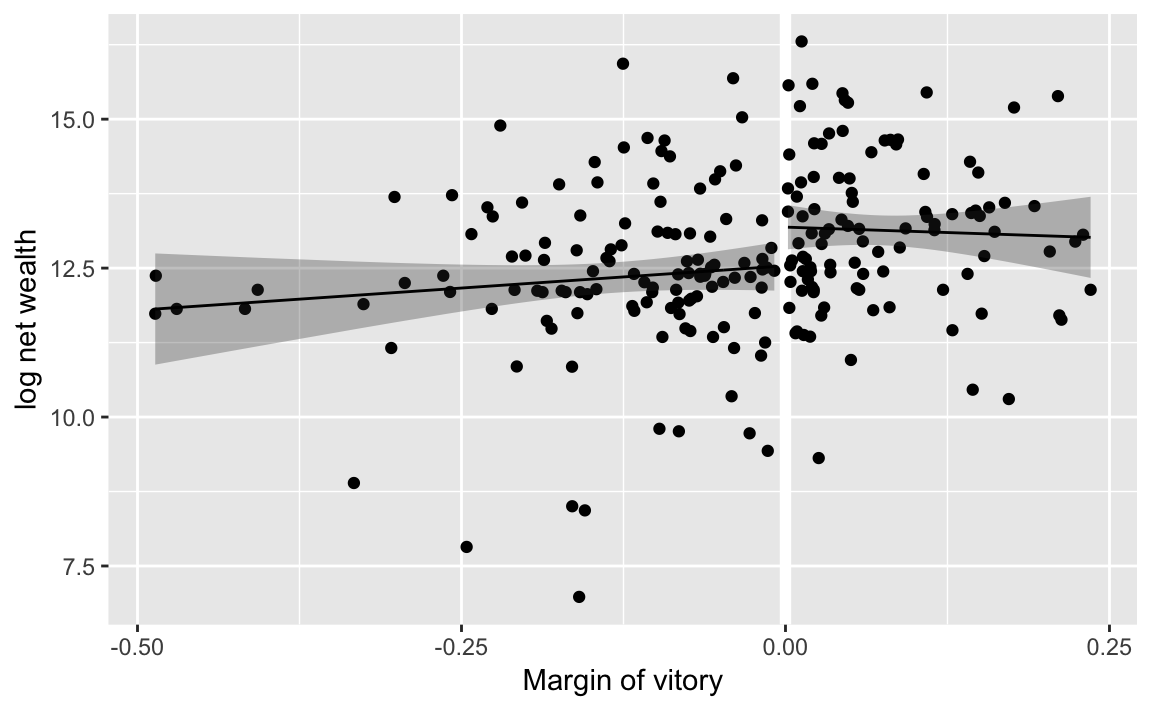
tory_y1 <- augment(tory_fit1, newdata = tibble(margin = 0))
tory_y1
#>   margin .fitted .se.fit
#> 1      0    12.5   0.214
tory_y0 <- augment(tory_fit2, newdata = tibble(margin = 0))
tory_y0
#>   margin .fitted .se.fit
#> 1      0    13.2   0.192
summary(tory_fit1)
#>
#> Call:
#> lm(formula = ln.net ~ margin, data = filter(MPs_tory, margin <
#>     0))
#>
#> Residuals:
#>    Min     1Q Median     3Q    Max
#> -5.320 -0.472 -0.035  0.663  3.580
#>
#> Coefficients:
#>             Estimate Std. Error t value Pr(>|t|)
#> (Intercept)   12.538      0.214   58.54   <2e-16 ***
#> margin         1.491      1.291    1.15     0.25
#> ---
#> Signif. codes:  0 '***' 0.001 '**' 0.01 '*' 0.05 '.' 0.1 ' ' 1
#>
#> Residual standard error: 1.43 on 119 degrees of freedom
#> Multiple R-squared:  0.0111, Adjusted R-squared:  0.00277
#> F-statistic: 1.33 on 1 and 119 DF,  p-value: 0.251
summary(tory_fit2)
#>
#> Call:
#> lm(formula = ln.net ~ margin, data = filter(MPs_tory, margin >
#>     0))
#>
#> Residuals:
#>    Min     1Q Median     3Q    Max
#> -3.858 -0.877  0.001  0.830  3.126
#>
#> Coefficients:
#>             Estimate Std. Error t value Pr(>|t|)
#> (Intercept)   13.188      0.192   68.69   <2e-16 ***
#> margin        -0.728      1.982   -0.37     0.71
#> ---
#> Signif. codes:  0 '***' 0.001 '**' 0.01 '*' 0.05 '.' 0.1 ' ' 1
#>
#> Residual standard error: 1.29 on 100 degrees of freedom
#> Multiple R-squared:  0.00135,    Adjusted R-squared:  -0.00864
#> F-statistic: 0.135 on 1 and 100 DF,  p-value: 0.714
Since we aren’t doing anything more with these values, there isn’t much benefit in keeping them in data frames.
# standard error
se_diff <- sqrt(tory_y0$.se.fit ^ 2 + tory_y1$.se.fit ^ 2)
se_diff
#> [1] 0.288
# point estimate
diff_est <- tory_y1$.fitted - tory_y0$.fitted
diff_est
#> [1] -0.65
# confidence interval
CI <- c(diff_est - se_diff * qnorm(0.975),
        diff_est + se_diff * qnorm(0.975))
CI
#> [1] -1.2134 -0.0859
# hypothesis test
z_score <- diff_est / se_diff
# two sided p value
p_value <- 2 * pnorm(abs(z_score), lower.tail = FALSE)
p_value
#> [1] 0.0239